Introduction
Standard CGE models are supply models that rely on the Walras hypothesis of perfect flexibility prices and quantities that ensures instantaneously the full and optimal use of production factors. Therefore, the assumption of perfect flexibility dismisses the existence of under-optimum equilibrium such as the presence of involuntary unemployment.
Contrarily to the previous Walrasian closure, prices in the Keynesian framework are rigid and therefore do not clear supply and demand. According to the Keynesian closure, the equality between supply and demand is satisfied by assuming that demand defines supply. According to this assumption, if there is no demand, there is no production. The law of Say does not hold as the level of demand defines the stock of production factors and not the contrary.
The two previous chapters have shown that these contrasting hypotheses have a very important impact on the properties of the model. The increase in public spending leads to: - a negative effect on the economy known as crowding out effect or eviction effect in the Walrasian framework (negative multiplier) - a positive effect on the economy known as crowding in effect in the Keynesian framework (positive multiplier)
The Walrasian and Keynesian closures have opposite drawbacks. Because of hypothesis of perfect flexibility of prices, Walrasian CGE are largely supply driven and neglect the role demand. On the contrary, with the hypothesis of the perfect price rigidity, Keynesian CGE are demand driven and neglect the impact of supply constrains on the level of production.
The assumption of perfect flexibility of prices and quantities appears more realistic in the long run than in the short run. Whereas the contrary is true for the assumption of perfect rigidity. Neo-Keynesian CGE models try to give a more realistic representation of the actual functioning of the economy by combining the advantages of the Walrasian and Keynesian closures: rigidity of prices and quantities in the short run but perfect flexibility in the long run. This amount to assuming slow adjustments of prices and quantities to their optimum, Neo-Keynesian closures have the advantage to allow for transitory or permanent under-optimum equilibrium.
Prices do not clear the markets and market ”imperfections” (e.g. involuntary unemployment) are taken into account. Prices and quantities are rigid in the short run and adjust slowly toward their (notional) optimal level. The notional level corresponds to the optimal (desired or target) level that an economic agent in question would choose in the absence of adjustment constraints.The general equilibrium is achieved by assuming that supply adjust to demand. In the short and medium run, situations of disequilibrium between notional supply and the actual supply and of under-utilization of the production capacity may occur.
In this chapter, we consider a small Neo-Keynesian model and investigate the impact of the same shock as the previous chapters: 1 percent GDP point increasing in public spending (G). Section 2 presents the model’s Neo-Keynesian closure while (Section 3) displays the simulation results both in the case of a closed economy and opened economy.
Model closure
Identities
Producers
Production
Production is defined by the market equilibrium condition between supply and demand. As in the Keynesian closure, production is endogenously determined as the sum of households consumption, investment and public spendings Équation 1:
\[Y = CH + I + G\]
Capital stock
The equation of capital stock in this closure Équation 5 is the same as the one introduced in the previous closures (but written slightly differently).
\[K = K_{t-1} \; \left( 1 - \delta \right) + I_{t-1}\]
The stock of capital in \(t\) is equal to the stock of capital in \(t-1\) minus the depreciated stock in \(t-1\) plus the investment occured in \(t-1\). In other words, the change in capital stock increases with the investment made in the previous period \(I_{t-1}\) and decreases with the depreciation of the capital stock (\(\delta.K_{t-1}\))
Capital cost
We assume that capital is entirely financed through bank credit and that the reimbursement of the debt corresponds to the depreciation of capital. The underlying ideas is that the loan cannot exceed the duration of the equipment. Assuming no capital gain, the cost of capital as defined in Équation 9 corresponds to the annuities paid by the firm (reimbursement of the debt plus interests paid).
\[c^{K} . K = p^{K}_{t-1} \; K_{t-1} \; \left( \delta + r^{K}_{t-1} \right)\]
Average price of the accumulated capital stock
Équation 10 provides the evolution of the value of the capital stock (and therefore of the debt) taking into account the value of past stock of capital (and its depreciation) and the value of past investment.
\[p^{K} . K = p^{K}_{t-1} \; K_{t-1} \; \left( 1 - \delta \right) + p_{t-1} \; I_{t-1}\]
Average interest rate paid on the debt
The average interest rate paid on debt Équation 11 is defined as the interest rate paid on the value of the accumulated capital stock (past capital stock net from its depreciation) and on past investment.
\[r^{K} . p^{K} . K = r^{K}_{t-1} \; p^{K}_{t-1} \; K_{t-1} \; \left( 1 - \delta \right) + p_{t-1} \; I_{t-1} \; r_{t-1}\]
Profit of firms (before investment)
The profit of firms before investment corresponds to the turn-over minus the labor and capital costs Équation 12.
\[PROF = p . Y - w . L - c^{K} . K\]
Firms’ savings
Firm’s savings Équation 13 are defined as a residual between profits on one hand and dividends (share of profits transferred to households) and investments on the other hand. If all profits are distributed as dividends, savings equal investment.
\[SAV^{F} = PROF - DIV - p . I\]
Firm’s bank debt
The firm’s bank debt Équation 14 depends positively on the amount of debt in the previous period (diminished by the part of debt reimbursed at the rate \(\varphi^{RD^{F}}_{t-1}\)) and negatively of the firm’s savings.
\[DEBT^{F} = DEBT^{F}_{t-1} \; \left( 1 - \varphi^{RD^{F}}_{t-1} \right) - SAV^{F}\]
Households
####Household’s income
The income of households includes incomes from labor and incomes from the dividends received from the firms.
\[INC = \left( w . L + DIV \right)\]
Household’s savings
Household’s savings depend positively on their income (net after tax deduction) and negatively on their consumption.
\[SAV^{H} = INC . \left( 1 - t^{inc} \right) - p . CH\]
Household’s total wealth
Household’s total wealth is defined as the sum of past stock of wealth and actual household’s savings.
\[WEALTH = WEALTH_{t-1} + SAV^{H}\]
Government and Central Bank
Government’s savings
The Government’s savings correspond to the tax income minus public spending, the reimbursement of the debt and interests paid.
\[SAV^{G} = t^{inc} . INC - p . G - DEBT^{G}_{t-1} \; \left( \varphi^{RD^{G}}_{t-1} + r^{DEBT,G}_{t-1} \right)\]
Total Government’s debt
Total government’s debt depends positively on the stock of debt in the previous period (diminished by the part of debt that is reimbursed) and negatively on government’s savings.
\[DEBT^{G} = DEBT^{G}_{t-1} \; \left( 1 - \varphi^{RD^{G}}_{t-1} \right) - SAV^{G}\]
Labor market
Unemployment rate
By definition, the unemployment rate Équation 27 is equal to the ratio between unemployed people and total labor force (sum of employed and unemployed people). The unemployment rate is an important determinant of the wages dynamic which is defined by a Phillips or a Wage Setting curve (detailed below in the section related to behavioral equations in the labor market) .
\[U = 1 - \frac{L}{LF}\]
Behavioral equations
Producers
Notional demand of factors
As explained in the previous chapters, the firm determines its demand for labor and capital by maximizing its profit, which is equivalent to minimizing its production costs assuming a given production function.
In the present closure, notional labor demand Équation 2 and notional capital demand Équation 3 are derived from a cost minimization assuming a CES function. However, contrarily to previous closures we do not assume that the price is equal to the cost because the firm’s mark-up is not necessary null (oligopoly competition; see chapter 1).
At the optimum, labor (capital) demand depends positively on the level of production negatively on productivity and on the relative cost of production factors.
Notional labor demand \[L^{n} = \left( \frac{Y}{PROG^{L}} \right) . \left( \left( \varphi^{L} \right) ^ {\rho^{KL}} \right) . \left( \frac{\left( \frac{w}{PROG^{L}} \right)}{c^{Y}} \right) ^ {\left( -\rho^{KL} \right)}\]
Notional capital demand \[K^{n} = \left( \frac{Y}{PROG^{K}} \right) . \left( \left( \varphi^{K} \right) ^ {\rho^{KL}} \right) . \left( \frac{\left( \frac{c^{K}}{PROG^{K}} \right)}{c^{Y}} \right) ^ {\left( -\rho^{KL} \right)}\]
Investment
Investment depends positively on the notional capital, the past investment and the ratio between the notional capital of the previous period and the capital stock of the previous period (gap between past effective capital and past notional capital), and depends negatively on real interest rate (calculated as the difference between nominal rate defined by the Central Bank and inflation). Coefficients before each variable in the right side of the equation stand for the elasticity between the dependant variable (Investment) and the corresponding independant variables.
\[\varDelta \left(\operatorname{log} I\right) = \alpha^{I,Kn} . \varDelta \left(\operatorname{log} K^{n}\right) + \alpha^{I,I1} . \varDelta \left(\operatorname{log} I_{t-1}\right) + \alpha^{I,KnK1} . \operatorname{log} \frac{K^{n}_{t-1}}{K_{t-1}} - \alpha^{I,rK} . \varDelta \left(r - \frac{\varDelta \left(p\right)}{p_{t-1}}\right)\]
Notional production price
Assuming imperfect (oligopolistic) competition and that the addressed demand to a firm is a negative function of its price, the optimal (notional) production price Équation 6 is defined as a mark-up over marginal production costs.
\[p^{n} . Y = c^{Y} . Y . \left( 1 + m^{up} \right)\]
Notional unit cost production cost
The notional unit cost of production Équation 8 is calculated as the weighted sum of the cost of labor (wage times notional labor) and the cost of capital (cost of capital times notional capital).
\[c^{Y} . Y = w . L^{n} + c^{K} . K^{n}\]
Notional mark-up
Prices are sensitive to the tension between supply and demand. In a Neo-Keynesian framework, when the demand is higher than the notional supply, producers still supply to satisfy the consumer’s demand but adjust their price (or mark-up) accordingly. This effect can be taken into account by assuming that the mark-up is a function of the gap between the effective and notional levels of production factors Équation 7. When the notional level of labor and capital is higher than the effective stock, the producer increases its mark-up, reflecting higher marginal cost faced by the producer when production capacities are too low. However, in the opposite case, when production capacities are too high, producers tend to decrease their mark-up in order to improve their competitiveness and attract clients.
\[\varDelta \left(\operatorname{log} \left(1 + m^{up,n}\right)\right) = \rho^{mupn,Ln} . \varDelta \left(\operatorname{log} \frac{L^{n}}{L}\right) + \rho^{mupn,Kn} . \varDelta \left(\operatorname{log} \frac{K^{n}}{K}\right)\]
Households
Notional households consumption
Households want to consume a constant share of their income (\(INC\)). As mentioned in Chapter 1, the propensity to save (\(\sigma\)) could be derived from an inter-temporal maximization of utility under revenue constraint like it is usually done in the standard neoclassical model (e.g. Romer, 2012).
\[CH^{n} . p = \left( 1 - \sigma \right) . INC . \left( 1 - t^{inc} \right)\]
Notional dividend for households
We assume that firms belong to households. In the long run, all profits are transferred them as dividend. The notional dividends going to Households are therefore equal to the firm’s profits (therefore at the steady state saving equal investment).
\[DIV^{n} = PROF\]
Notional propensity to save equation
In order to account for inter-temporal maximization behaviour of certain consumers, the desired saving rate may depend positively on the real interest rate as predicted by the permanent income hypothesis1 Friedman (1957) and positively on the Government’s debt ratio as predicted by the Ricardian equivalence2 Ricardo (1888) and Buchanan (1976) and negatively on the unemployment rate3. The increase in unemployment leads to a decrease in income. Because of consumption habits, the decrease in consumption is generally lower than the decrease in income. This leads to a decrease of the actual saving rate.
\[\varDelta \left(\operatorname{log} \left(1 - \sigma^{n}\right)\right) = \rho^{\sigma,U} . \varDelta \left(U\right) - \rho^{\sigma,r} . \varDelta \left(r\right) + \rho^{\sigma,p} . \varDelta \left(\frac{\varDelta \left(p\right)}{p_{t-1}}\right) - \rho^{\sigma,DEBT} . \varDelta \left(\operatorname{log} \left(\frac{DEBT^{G}}{\left( p . Y \right)}\right)\right)\]
The ambiguous relationship between savings and the interest rate.Econometric studies failed to establish a clear empirical relationship between interest rates and the saving behavior of households Gylfason (1993). Many studies reported significantly positive effects of interest rates on saving propensities in several countries. Others have concluded that no such evidence, while some others indicated an inverse relationship between saving propensities and interest rate. An overview of the results regarding the relationship between both variables for 24 studies, mainly covering the USA, are displayed in Gylfason (1993).
Half of the studies failed to corroborate a significantly positive relationship between interest rates and savings. The remaining others indicate a fairly strong positive link between interest rates and saving (with an elasticity coefficient of 0.7).
Gylfason (1993) argues that an elasticity of substitution above unity is necessary to derive a negative relationship between consumption and interest in the simple model considered. But an elasticity of substitution below unity implies a positive relationship between the two.
The interdependence of saving and interest rates within the economic system allows for the possibility of them moving in the same direction or in opposite directions over time and across countries Gylfason (1993). This direction is influenced by exogenous variables that impact both variables. Despite the structural links between saving and interest derived from the neoclassical theory of inter-temporal choice have proven hard to establish in econometric research. It is still possible to proof how saving and interest rates may seem to be negatively correlated in economic data despite a strongly positive structural link between.
Government and Central Bank
Notional interest rate of the Central Bank (Taylor reaction function)
The interest rate is set by the Central Bank (CB) according to a Taylor reaction function of the central bank Taylor (1993): the real interest rate is a positive function of inflation and a negative function of the unemployment rate (\(U\)). The fact that the Central Bank determines the interest rate level based on inflation and unemployment has an effect on the demand via the negative effect of the real interest rate on consumption and investment. Thus, the interest rate is not determined by the equilibrium between investment and saving as assumed in Walrasian CGE models (see e.g. Shoven and Whalley, 1992).
\[\varDelta \left(r^{n}\right) = \rho^{rn,p} . \varDelta \left(\frac{\varDelta \left(p\right)}{p_{t-1}}\right) - \rho^{rn,U} . \varDelta \left(U\right)\]
Taylor reaction function. The objective function of the Central Bank (\(O\)) is to minimize the deviations of inflation \(Inf\) from its target level \(Inf_{t}\) which is called inflation gap \(Inf_{g}\) and unemployment \(U\) from its target level \(U_{t}\) known as unemployment gap \(U_{g}\). Unemployment is used as a measure of output activity. Assuming that this objective function is quadratic, its general form can be expressed as follows:
\[O = a.(Inf-Inf_{t})^{2} + b. (U-U_{t})^{2} = a.(Inf_{g})^{2} + b. (U_{g})^{2}\]
To minimize \(O\), we set partial derivatives to 0:
\[\frac{\partial O}{\partial Inf_{g}}= 0 \Longleftrightarrow \frac{\partial O}{\partial Inf_{g}}= 2a.Inf_{g} = 0 \Longleftrightarrow Inf_{g}= 0 \]
\[\frac{\partial O}{\partial U_{g}}= 0 \Longleftrightarrow \frac{\partial O}{\partial U_{g}}= 2a.U_{g} = 0 \Longleftrightarrow U_{g}= 0\] Which means that at the optimal level, there is neither inflation gap nore output or unemployment gap. Assuming a linear relationship between the iterest rate on the one hand and inflation rate \(Inf\) and Unemployment \(U\) on the other hand, we can write:
\[r = \rho_{0} + \rho_{1}.Inf + \rho_{2}.U\]
with \(\rho*{0} = -*\rho{1}.Inf\_{0} - \rho*{2}.U*{0}\), we can write:
\[r = \rho_{1}.(Inf- Inf_{0}) + \rho_{2}.(U-U_{0})\]
With the derivative, we get:
\[ \Delta(r)= \rho_{0} + \rho_{1}.\Delta(Inf) + \rho_{2}.\Delta(U)\]
As \(\Delta(\rho_{0}) = -\rho_{1}.\Delta(Inf_{0}) - \rho_{2}.\Delta(U_{0}) = 0\), we can write:
\[\Delta(r)= \rho_{1}.\Delta(Inf) + \rho_{2}.\Delta(U)\]
Notional income tax rate
The notional income tax rate is positively related to the ratio of debt to GDP. Higher debt to GDP ratio may put pressure on the government’s finances, increasing the amount of interests to pay. Therefore, increasing income taxes which constitutes a major source of revenue may help paying back the government’s debt.
\[\varDelta \left(t^{inc,n}\right) = \rho^{tinc,debt} . \varDelta \left(\frac{DEBT^{G}}{\left( p . Y \right)}\right)\]
Notional income tax rate. A common objective of governments is to maximize social welfare that takes into account various factors. The government may aim to allocate resources and set tax policies in a way that maximizes overall social welfare. It may also aim at minimizing the fiscal deficit or reducing the debt-to-GDP ratio.The optimal budgetary rule is then determined by solving an optimization problem based on the chosen objective function, subject to various constraints. The specific mathematical expressions and solution of the government’s objective function can be complex and depend on several factors. Herein, we present simple steps to the problem.
In a simple way, let’s assume that the government’s objective is to maximize social welfare, which can be represented by a utility function \(U(G, t_{\text{inc}})\), where \(G\) is the level of public goods provided by the government, and \(t_{\text{inc}}\) is the income tax rate.
The government’s tax revenue is determined by the income tax rate and the level of taxable income in the economy. Let’s denote tax revenue as \(\text{REV}(t_{\text{inc}})\). The government must satisfy a budget constraint that relates tax revenue to government spending, which can be represented as \(\text{REV}(t_{\text{inc}}) = G\).
The government seeks to maximize its objective function \(U(G, t_{\text{inc}})\) subject to the budget constraint \(\text{REV}(t_{\text{inc}}) = G\).
Introducing the Lagrangian to solve the optimisation problem we can wirte:
\[L = U(G, t_{\text{inc}}) + \lambda(G - \text{REV}(t_{\text{inc}}))\]
To find the income tax rate \(t_{\text{inc}}\) that maximizes the government’s objective function while satisfying the budget constraint, We calculate partial derivatives of the Lagrangian with respect to \(G\), \(t_{\text{inc}}\), and \(\lambda\), and set them equal to zero to find the optimal values.
Defining a specific functional form of the objective functions and including more variable in the constraints will lead to a more complex but complete demonstration.
Average interest rate paid on the total Government’s debt
The average interest rate paid on the total Government’s debt follows the evolution of the interest rate of the CB. In other words, the gap between the two interest rates is constant, reflecting the assumption of a constant risk premium.
\[\varDelta \left(r^{DEBT,G}\right) = \varDelta \left(r\right)\]
Labor market
Notional wage (WS or Plillips curve)
In neo-Keynesian models, the wage do not clear the labor. The wage equation is often defined as a Phillips or Wage Setting (WS) curve Blanchard et Katz (1999) and Heyer et al. (2007). Wages increase with inflation and decrease with the unemployment rate. This specification leads to an increase (resp. decrease) in inflation if the unemployment rate is higher (resp. lower) than the equilibrium rate of unemployment.
The equation of wage depends positively on the notional wage and on the effective wage in the previous period and negatively on the the ratio of the wage in the previous period and the notional wage in the previous period also.
\[\varDelta \left(\operatorname{log} w^{n}\right) = \rho^{wn} + \rho^{wn,pe} . \varDelta \left(\operatorname{log} p^{e}\right) + \rho^{wn,PROGL} . \varDelta \left(\operatorname{log} PROG^{L}\right) - \rho^{wn,U} . U - \rho^{wn,dU} . \varDelta \left(U\right)\]
The Phillips curve. A derivation of the Phillips curve can be found in Ball et Moffitt (2001):
We denote inflation by \(\pi\) and wage inflation by \(\omega\), so real wage growth is \(\omega - \pi\). We assume that wage setters have a target for real-wage growth given by the following equation:
\[(\omega - \pi)^* = \alpha - \gamma U + \delta \theta + (1 - \delta)A + \eta, \quad \alpha, \gamma > 0, \quad 0 \leq \delta \leq 1\]
with \(U\) is unemployment, \(\theta\) is labor productivity growth, \(A\) is an aspiration wage increase and \(\eta\) is an error term.
The underlying assumptions of this equation assume a negative relationship between unemployment and the target real wage growth and a positive influence of productivity growth and aspiration wage on the target real wage growth. The aspiration wage increase \(A\) given by :
\[A=\frac{1-\beta}{\beta} \sum_{i=1}^{\infty} \beta^i(\omega-\pi)_{-i}\]
To interpret these two equations, two extreme cases can be considered: - \(\delta =1\) : this is a neoclassical benchmark in which productivity growth feeds one-for-one into wages, and aspirations are irrelevant. - \(\delta =0\) : in this case, productivity is irrelevant and wage increases are based on aspirations.
Period’s aspiration for a real-wage increase is a weighted average of past increases, with exponentially declining weights. Aspiration real-wage increase can also be written recursively as follows:
\[A =\beta A_{-1}+(1-\beta)(\omega-\pi)_{-1}\]
We assume that productivity growth and past real-wage growth influence wage setting and that the sum of their coefficients equals to 1.The target depends one-for-one on productivity growth in a steady state with real-wage growth equal to productivity growth.
Wage setters must choose nominal wages one period in advance.They choose a nominal increase \(\omega\) equal to their target real wage increase, \((\omega-\pi)^*\), plus expected inflation. Expected inflation equals last period’s inflation \((\pi_{-1})\).
Combining these assumptions with the first equation of target real-wage growth gives the following “Wage Phillips curve”:
\[\omega=\alpha+\pi_{-1}-\gamma U+\delta \theta+(1-\delta) A+\eta\]
Adjustments
The hypothesis of slow adjustments of prices and quantities is an important feature of neo-Keynesian models that distinguishes them from Walrasien CGE models.
In a neo-Keynesian framework, firms do not adjust instantaneously their price or their inputs (labor, capital, intermediary consumption) to the new optimum level after a shock in the economy. The same holds for the consumption of households, the wage setting or the adjustment of the interest rate. These slow adjustments result from rational decisions in the presence of various adjustment constrains.
The changes in consumption patterns are also the result of a slow process. The fact that the consumption of households follows income with lags is known as an old empirical observation Tinbergen (1942). Several consumption theories have been proposed to explain the slow adjustment of consumption to income observed empirically.
Many studies have shown empirically that prices adjust slowly Carlton (1986), Cecchetti (1985) and Kashyap (1995). To take into account that the changes in price are all the more costly that they are large (large increases are less accepted by consumers than small increases), Rotemberg (1982), Tinsley (2002) propose to use quadratic adjustment cost models. The firm defines the optimal price as a trade-off between the cost of adjusting and the cost of not been adjusted.
The specification of the price and quantity equations assume that firms gradually adjust their effective price and quantity to the optimal level. Adjustment models provide a microeconomic foundation for the specification of the adjustment process we have selected by deriving the adjustment process from an optimal behavior. Initially developed by Eisner et Strotz (1963) and Gould (1968), these models were extended by several authors including Lucas (1967), Schramm (1970) and Treadway (1971). We derive below the static case which deliver the same adjustment equation derived from the inter-temporal model proposed by Rotemberg (1982).
Adjustment models generally assume a continuous relation between the objective function \(\Gamma\) of the agent (i.e. the profit for a firm, the utility for the consumer, the Government or the Central Bank) and the variable \(X\) controlled by the agent (i.e. price, input demand, consumption, interest rate, tax rate, etc): \(\Gamma_t\left(X_t\right)\). The notional (i.e. optimal or desired) profit (or utility) is then written \(\Gamma_t\left(X_t^n\right)\) where \(n\) denotes the level desired by firms. At the neighborhood of the optimum, the second-order approximation of the difference between the effective and desired profits is written:
Minimizing an adjustment cost function
\[ \Gamma_t\left(X_t\right)-\Gamma_t\left(X_t^n\right)=\Gamma_t^{\prime}\left(X_t^n\right)\left(X_t-X_t^n\right)+\Gamma_t^{\prime \prime}\left(X_t^n\right)\left(X_t-X_t^n\right)^2\]
The profit being maximum for \(X_t^n, \Gamma_t^{\prime}\left(X_t^n\right)=0\) and \(\Gamma_t^{\prime \prime}\left(X_t^n\right)<0\). As a first approximation, the adjustment cost, i.e. the loss of profit suffered by a company that is not in the optimum, is therefore:
\[C_D=\Gamma_t\left(X_t^n\right)-\Gamma_t\left(X_t\right)=C_D\left(X_t-X_t^n\right)^2\]
Where: \[ C_D=-\Gamma_t^{\prime \prime}\left(X_t^n\right)\]
Suppose that the adjustment cost is proportional to the square of the speed of adjustment:
\[C_A=c_A\left(X_t-X_{t-1}\right)^2\]
Where:
\[c_A>0\]
Minimizing the total cost function \(\left(C_t=C_D+C_A\right)\) is equivalent to solving:
\[C_t^{\prime}\left(X_t\right)=2 c_D\left(X_t-X_t^n\right)+2 c_A\left(X_t-X_{t-1}\right)=0\]
The condition of the second order \(\left(C_t^{\prime \prime}\left(X_t\right)>0\right)\) being always verified, the optimal adjustment which minimizes the total cost has the following dynamic process:
\[ X_t=\alpha X_t^n+(1-\alpha) X_{t-1}\]
With:
\[\alpha=\frac{c_D}{\left(c_D+c_A\right)}\]
With this simple model, the average adjustment time is:
\[\frac{\alpha}{(1-\alpha)}=\frac{c_D}{c_A}\]
The slower the adjustment, the higher the adjustment cost \(c_A\) compared to the cost of non being adjusted \(c_D\).
Examples of adjustment
Equation (2.1) describes an arithmetic adjustment process: \(X_t\) is arithmetic weighed average of its notional value and past value and therefore converges dynamically to it notional value if the latter is stationary. We may use it for variable that are stationary in the long run (e.g. the interest rate). When the variable is not stationary, equation (2.1) does not guaranty that the variable reach its notional value in the long run. It is then preferable to write the adjustment process in log form and to include expectation. Herein two examples of adjustment equations with anticipations Where \(Xe\) is the expected (anticipated) value of X at period t. We assume that the anticipations are adaptive (backward-looking):
Equation of production price \[\operatorname{log} p = \alpha^{P,Pn} . \operatorname{log} p^{n} + \left( 1 - \alpha^{P,Pn} \right) . \left( \operatorname{log} p_{t-1} + \varDelta \left(\operatorname{log} p^{e}\right) \right)\]
Expected production price inflation \[\varDelta \left(\operatorname{log} p^{e}\right) = \alpha^{Pe,Pe1} . \varDelta \left(\operatorname{log} p^{e}_{t-1}\right) + \alpha^{Pe,P1} . \varDelta \left(\operatorname{log} p_{t-1}\right) + \alpha^{Pe,Pn} . \varDelta \left(\operatorname{log} p^{n}\right)\]
Households final consumption \[\operatorname{log} CH = \alpha^{CH,CHn} . \operatorname{log} CH^{n} + \left( 1 - \alpha^{CH,CHn} \right) . \left( \operatorname{log} CH_{t-1} + \varDelta \left(\operatorname{log} CH^{e}\right) \right)\]
Expected households final consumption growth \[\varDelta \left(\operatorname{log} CH^{e}\right) = \alpha^{CHe,CHe1} . \varDelta \left(\operatorname{log} CH^{e}_{t-1}\right) + \alpha^{CHe,CH1} . \varDelta \left(\operatorname{log} CH_{t-1}\right) + \alpha^{CHe,CHn} . \varDelta \left(\operatorname{log} CH^{n}\right)\]
The constraint \(\alpha^{CHe,CHe1} + \alpha^{CHe,CH1}+\alpha^{CHe,CHn} = 1\) ensures that in the long run expectations are accurate.
Equation of interest rate (example of adjustment without anticipated value) \[r = \alpha^{r} . r^{n} + \left( 1 - \alpha^{r} \right) . r_{t-1}\]
Exception in the adjustment process: example of the wage equation \[\varDelta \left(\operatorname{log} w\right) = \alpha^{W,Wn} . \varDelta \left(\operatorname{log} w^{n}\right) + \alpha^{W,W1} . \varDelta \left(\operatorname{log} w_{t-1}\right) - \alpha^{W,W1Wn1} . \operatorname{log} \frac{w_{t-1}}{w^{n}_{t-1}}\]
Simulation results
Before presenting some main results regarding the impact on public spendings of one GDP point considering a Neo-Keynesian closure, we first display the main conclusions regarding the effect of the same shock in the case of a Walrasian and Keynesian models.
Main impacts of a shock on G in the Walrasian closure (revision)
- Negative multiplier due to a crowding out effect: rising public expenditures reduces private expenditures (households consumption and investment).
- Production is determined by capital and labor. Labor is exogenous and capital defined by the previous year investment and depreciation.
- Therefore, no room for additional production (no spare production capacity). Increasing public consumption is only possible if investment and household’s consumption decreases.
- A lower investment leads to a the future capital stock, increasing the interest rate.
- As capital decreases, production also decreases in the following period.
- As production decreases, wages have to decrease to maintain full employment.
- Vicious negative cycle
Main impacts of a shock on G in the Keynesian closure (revision)
- Positive multiplier: the increase in public spending has an immediate positive effect on the economy
- The supply constraint is no more held: production is no more predetermined by labor and capital
- Implicit assumption of spare production capacity
- As production increases, more factors are needed which increases demand for labor and capital.
- Increasing labor and capital rises production which increases consumption and investment
Main impacts of a shock on G in the Neo-Keynesian closure
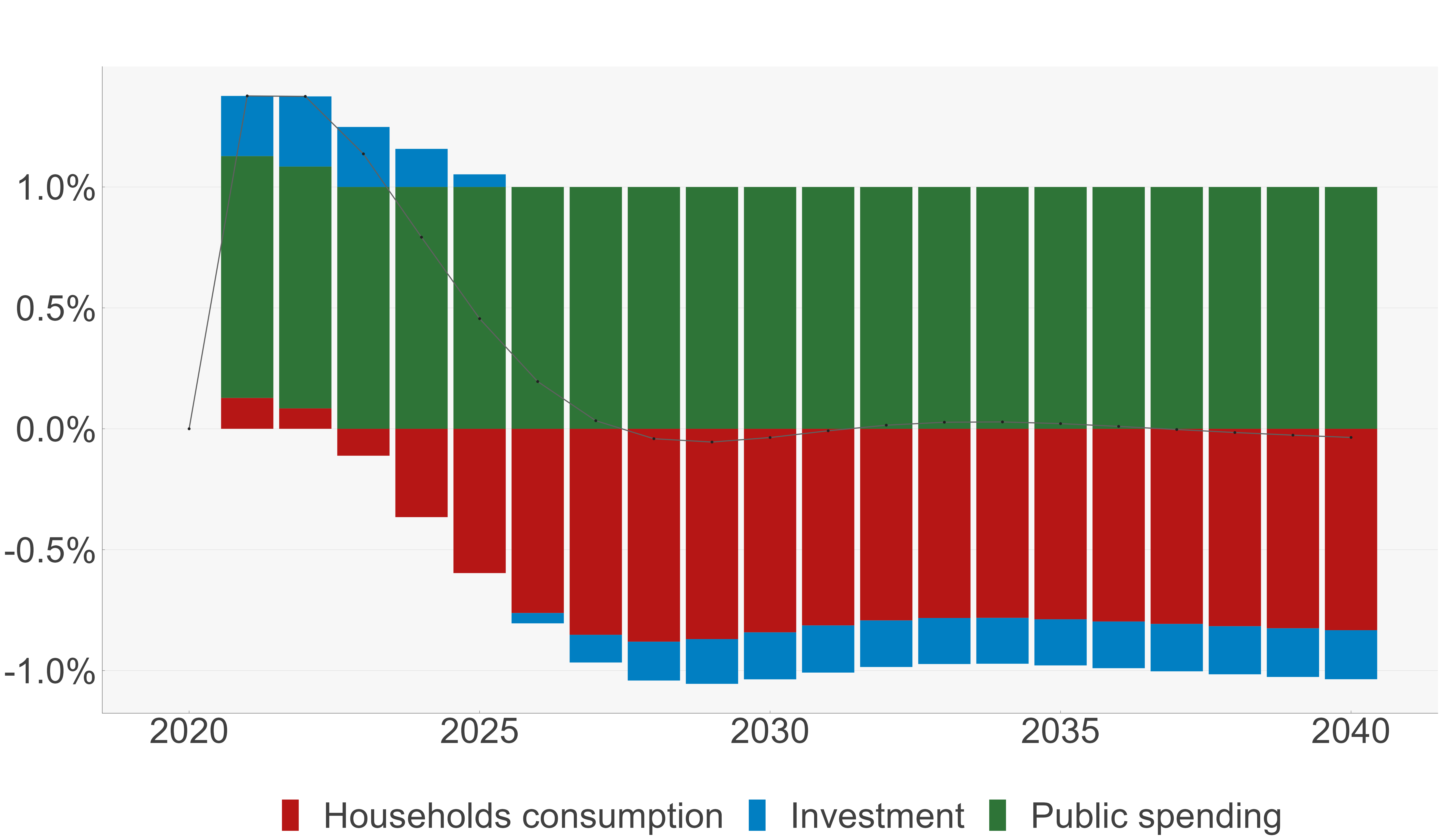
- An increase in public spending has an immediate positive effect on production (Figure 1). The increase in production decreases unemployment as more labor is required for production
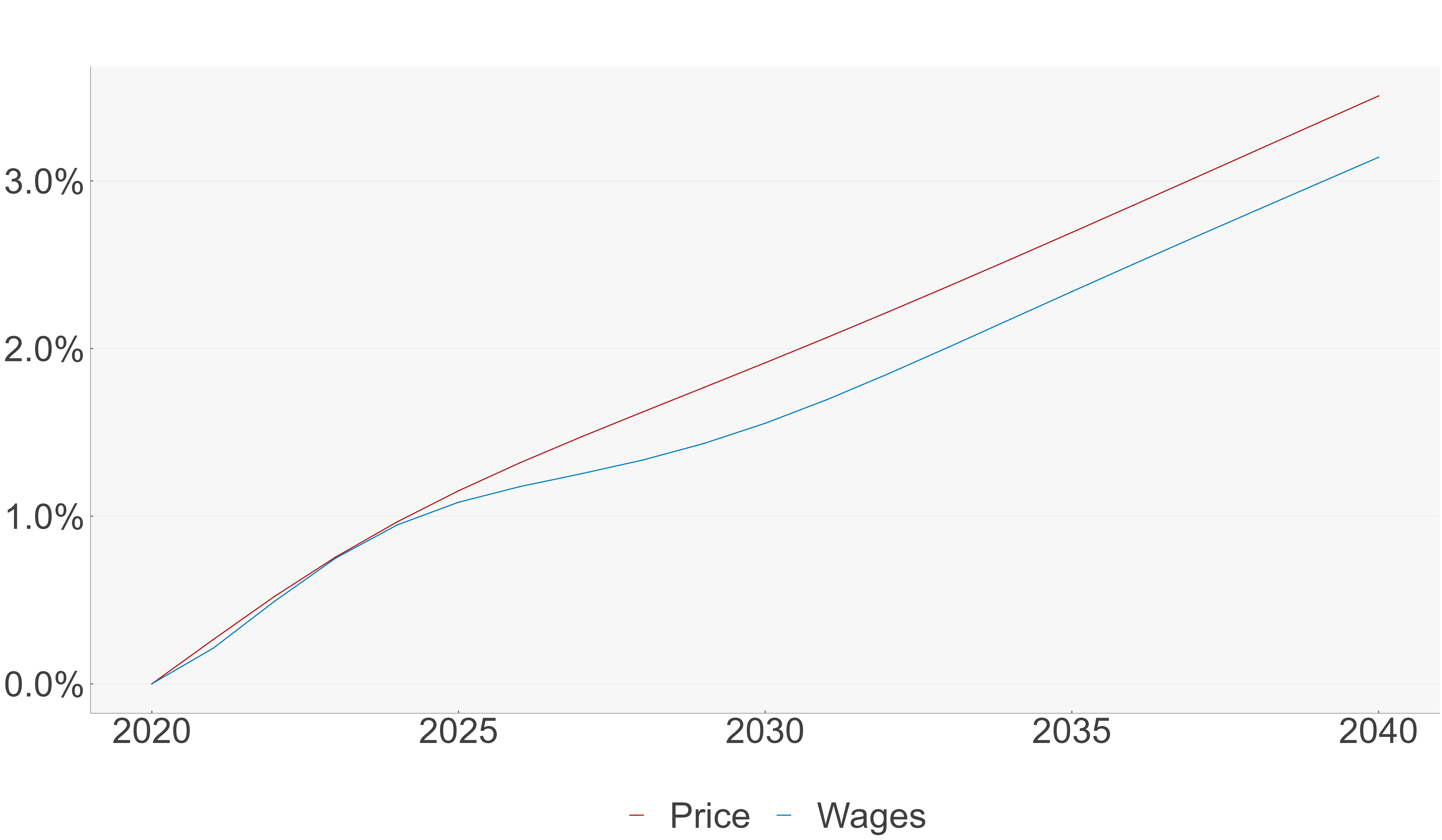
- Lower unemployment rises demand which puts upward pressure on prices and generates inflation (Figure 2).
- Because of the negative relationship between unemployment and wages (Phillips curve), wages increase also (Figure 2), which increases the cost of production, prices and mark-up
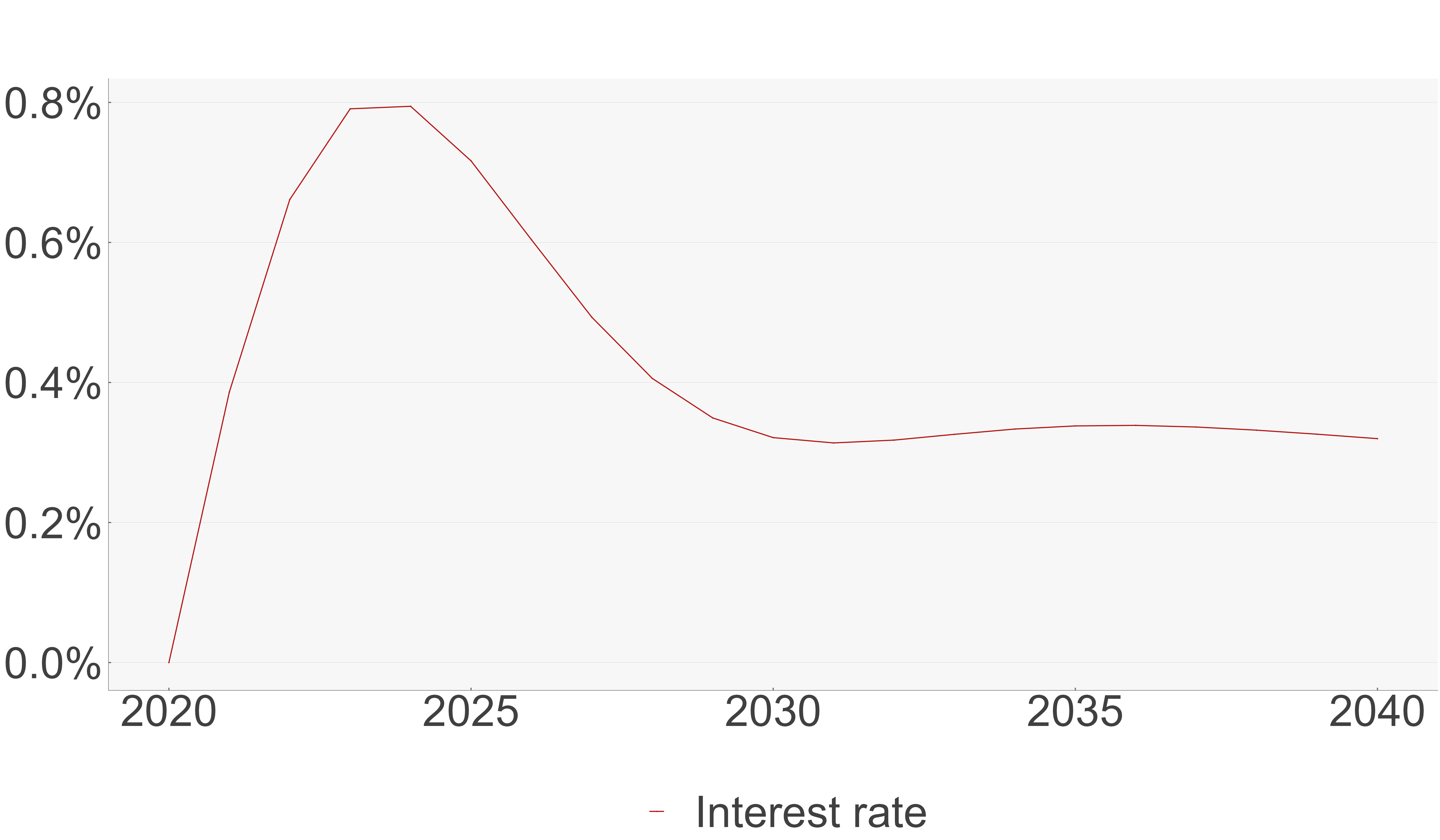
- Because of the negative relationship between unemployment and interest rate, the decrease of unemployment increases interest rates (Taylor reaction function) (Figure 3), which decreases investment.
- As interest rate increase, savings increase (we assume that savings are accumulated without precising where they are invested in the economy) but consumption decreases.
- As investment and consumption decrease because of the inflationist pressure driven by higher production, there is a crowding out effect. On the long run, the effect on GDP is null.
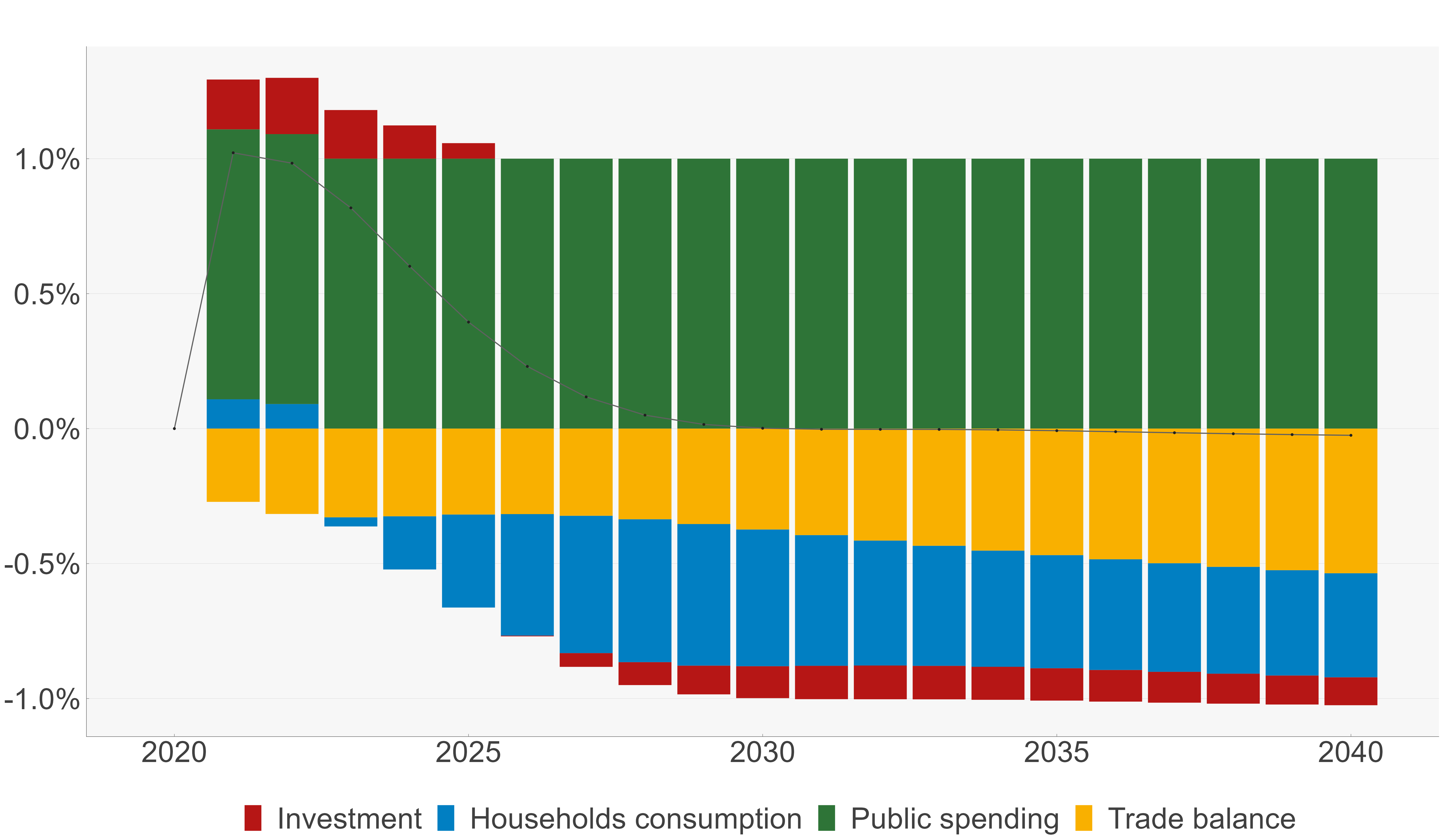
- Case of an open economy (same shock on G): positive multiplier in the short run but effect null on GDP on the long run (eviction effect due to consumption and trade balance (Figure 4)
Annexes
Endogenous variables’ equations
Producers
Production (GDP) \[Y = CH + I + G \tag{1}\]
Notional labor demand \[L^{n} = \left( \frac{Y}{PROG^{L}} \right) . \left( \left( \varphi^{L} \right) ^ {\rho^{KL}} \right) . \left( \frac{\left( \frac{w}{PROG^{L}} \right)}{c^{Y}} \right) ^ {\left( -\rho^{KL} \right)} \tag{2}\]
Notional capital demand \[K^{n} = \left( \frac{Y}{PROG^{K}} \right) . \left( \left( \varphi^{K} \right) ^ {\rho^{KL}} \right) . \left( \frac{\left( \frac{c^{K}}{PROG^{K}} \right)}{c^{Y}} \right) ^ {\left( -\rho^{KL} \right)} \tag{3}\]
Investment \[\varDelta \left(\operatorname{log} I\right) = \alpha^{I,Kn} . \varDelta \left(\operatorname{log} K^{n}\right) + \alpha^{I,I1} . \varDelta \left(\operatorname{log} I_{t-1}\right) + \alpha^{I,KnK1} . \operatorname{log} \frac{K^{n}_{t-1}}{K_{t-1}} - \alpha^{I,rK} . \varDelta \left(r - \frac{\varDelta \left(p\right)}{p_{t-1}}\right) \tag{4}\]
Capital stock \[K = K_{t-1} \; \left( 1 - \delta \right) + I_{t-1} \tag{5}\]
Notional production price \[p^{n} . Y = c^{Y} . Y . \left( 1 + m^{up} \right) \tag{6}\]
Notional mark-up \[\varDelta \left(\operatorname{log} \left(1 + m^{up,n}\right)\right) = \rho^{mupn,Ln} . \varDelta \left(\operatorname{log} \frac{L^{n}}{L}\right) + \rho^{mupn,Kn} . \varDelta \left(\operatorname{log} \frac{K^{n}}{K}\right) \tag{7}\]
Notional unit cost production cost \[c^{Y} . Y = w . L^{n} + c^{K} . K^{n} \tag{8}\]
Capital cost \[c^{K} . K = p^{K}_{t-1} \; K_{t-1} \; \left( \delta + r^{K}_{t-1} \right) \tag{9}\]
Average price of the accumulated capital stock \[p^{K} . K = p^{K}_{t-1} \; K_{t-1} \; \left( 1 - \delta \right) + p_{t-1} \; I_{t-1} \tag{10}\]
Average interest rate paid on the debt \[r^{K} . p^{K} . K = r^{K}_{t-1} \; p^{K}_{t-1} \; K_{t-1} \; \left( 1 - \delta \right) + p_{t-1} \; I_{t-1} \; r_{t-1} \tag{11}\]
Profit of firms (before investment) \[PROF = p . Y - w . L - c^{K} . K \tag{12}\]
Firms’ savings \[SAV^{F} = PROF - DIV - p . I \tag{13}\]
Firms’ bank debt \[DEBT^{F} = DEBT^{F}_{t-1} \; \left( 1 - \varphi^{RD^{F}}_{t-1} \right) - SAV^{F} \tag{14}\]
Households
Notional households consumption \[CH^{n} . p = \left( 1 - \sigma \right) . INC . \left( 1 - t^{inc} \right) \tag{15}\]
Households’ income \[INC = \left( w . L + DIV \right) \tag{16}\]
Notional dividend for households \[DIV^{n} = PROF \tag{17}\]
Notional propensity to save equation \[\varDelta \left(\operatorname{log} \left(1 - \sigma^{n}\right)\right) = \rho^{\sigma,U} . \varDelta \left(U\right) - \rho^{\sigma,r} . \varDelta \left(r\right) + \rho^{\sigma,p} . \varDelta \left(\frac{\varDelta \left(p\right)}{p_{t-1}}\right) - \rho^{\sigma,DEBT} . \varDelta \left(\operatorname{log} \left(\frac{DEBT^{G}}{\left( p . Y \right)}\right)\right) \tag{18}\]
Households’ savings \[SAV^{H} = INC . \left( 1 - t^{inc} \right) - p . CH \tag{19}\]
Households’ total wealth \[WEALTH = WEALTH_{t-1} + SAV^{H} \tag{20}\]
Government and Central Bank
Notional interest rate of the Central Bank (Taylor reaction function) \[\varDelta \left(r^{n}\right) = \rho^{rn,p} . \varDelta \left(\frac{\varDelta \left(p\right)}{p_{t-1}}\right) - \rho^{rn,U} . \varDelta \left(U\right) \tag{21}\]
Notional income tax rate \[\varDelta \left(t^{inc,n}\right) = \rho^{tinc,debt} . \varDelta \left(\frac{DEBT^{G}}{\left( p . Y \right)}\right) \tag{22}\]
Government’s savings \[SAV^{G} = t^{inc} . INC - p . G - DEBT^{G}_{t-1} \; \left( \varphi^{RD^{G}}_{t-1} + r^{DEBT,G}_{t-1} \right) \tag{23}\]
Average interest rate paid on the total Government’s debt \[\varDelta \left(r^{DEBT,G}\right) = \varDelta \left(r\right) \tag{24}\]
Total Government’s debt \[DEBT^{G} = DEBT^{G}_{t-1} \; \left( 1 - \varphi^{RD^{G}}_{t-1} \right) - SAV^{G} \tag{25}\]
Labor market
Notional wage (WS or Phillips curve) \[\varDelta \left(\operatorname{log} w^{n}\right) = \rho^{wn} + \rho^{wn,pe} . \varDelta \left(\operatorname{log} p^{e}\right) + \rho^{wn,PROGL} . \varDelta \left(\operatorname{log} PROG^{L}\right) - \rho^{wn,U} . U - \rho^{wn,dU} . \varDelta \left(U\right) \tag{26}\]
Unemployment rate \[U = 1 - \frac{L}{LF} \tag{27}\]
Adjustments
Wage \[\varDelta \left(\operatorname{log} w\right) = \alpha^{W,Wn} . \varDelta \left(\operatorname{log} w^{n}\right) + \alpha^{W,W1} . \varDelta \left(\operatorname{log} w_{t-1}\right) - \alpha^{W,W1Wn1} . \operatorname{log} \frac{w_{t-1}}{w^{n}_{t-1}} \tag{28}\]
Production price \[\operatorname{log} p = \alpha^{P,Pn} . \operatorname{log} p^{n} + \left( 1 - \alpha^{P,Pn} \right) . \left( \operatorname{log} p_{t-1} + \varDelta \left(\operatorname{log} p^{e}\right) \right) \tag{29}\]
Expected production price inflation \[\varDelta \left(\operatorname{log} p^{e}\right) = \alpha^{Pe,Pe1} . \varDelta \left(\operatorname{log} p^{e}_{t-1}\right) + \alpha^{Pe,P1} . \varDelta \left(\operatorname{log} p_{t-1}\right) + \alpha^{Pe,Pn} . \varDelta \left(\operatorname{log} p^{n}\right) \tag{30}\]
Households final consumption \[\operatorname{log} CH = \alpha^{CH,CHn} . \operatorname{log} CH^{n} + \left( 1 - \alpha^{CH,CHn} \right) . \left( \operatorname{log} CH_{t-1} + \varDelta \left(\operatorname{log} CH^{e}\right) \right) \tag{31}\]
Expected households final consumption growth \[\varDelta \left(\operatorname{log} CH^{e}\right) = \alpha^{CHe,CHe1} . \varDelta \left(\operatorname{log} CH^{e}_{t-1}\right) + \alpha^{CHe,CH1} . \varDelta \left(\operatorname{log} CH_{t-1}\right) + \alpha^{CHe,CHn} . \varDelta \left(\operatorname{log} CH^{n}\right) \tag{32}\]
Labor \[\operatorname{log} L = \alpha^{L,Ln} . \operatorname{log} L^{n} + \left( 1 - \alpha^{L,Ln} \right) . \left( \operatorname{log} L_{t-1} + \varDelta \left(\operatorname{log} L^{e}\right) \right) \tag{33}\]
Expected labor growth \[\varDelta \left(\operatorname{log} L^{e}\right) = \alpha^{Le,Le1} . \varDelta \left(\operatorname{log} L^{e}_{t-1}\right) + \alpha^{Le,L1} . \varDelta \left(\operatorname{log} L_{t-1}\right) + \alpha^{Le,Ln} . \varDelta \left(\operatorname{log} L^{n}\right) \tag{34}\]
Dividend for households \[\operatorname{log} DIV = \alpha^{DIV,DIVn} . \operatorname{log} DIV^{n} + \left( 1 - \alpha^{DIV,DIVn} \right) . \left( \operatorname{log} DIV_{t-1} + \varDelta \left(\operatorname{log} DIV^{e}\right) \right) \tag{35}\]
Expected dividend for households \[\varDelta \left(\operatorname{log} DIV^{e}\right) = \alpha^{DIVe,DIVe1} . \varDelta \left(\operatorname{log} DIV^{e}_{t-1}\right) + \alpha^{DIVe,DIV1} . \varDelta \left(\operatorname{log} DIV_{t-1}\right) + \alpha^{DIVe,DIVn} . \varDelta \left(\operatorname{log} DIV^{n}\right) \tag{36}\]
Interest rate of the Central Bank \[r = \alpha^{r} . r^{n} + \left( 1 - \alpha^{r} \right) . r_{t-1} \tag{37}\]
Propensity to save \[\sigma = \alpha^{\sigma} . \sigma^{n} + \left( 1 - \alpha^{\sigma} \right) . \sigma_{t-1} \tag{38}\]
Mark-up \[m^{up} = \alpha^{m,up} . m^{up,n} + \left( 1 - \alpha^{m,up} \right) . m^{up}_{t-1} \tag{39}\]
Income tax rate \[t^{inc} = \alpha^{t,inc} . t^{inc,n} + \left( 1 - \alpha^{t,inc} \right) . t^{inc}_{t-1} \tag{40}\]
Glossary of variables
| \(c^{K}\) | Capital cost | 9 |
| \(c^{Y}\) | Notional unit cost production cost | 8 |
| \(CH\) | Households final consumption | 31 |
| \(CH^{e}\) | Expected households final consumption growth | 32 |
| \(CH^{n}\) | Notional households consumption | 15 |
| \(DEBT^{F}\) | Firms’ bank debt | 14 |
| \(DEBT^{G}\) | Total Government’s debt | 25 |
| \(DIV\) | Dividend for households | 35 |
| \(DIV^{e}\) | Expected dividend for households | 36 |
| \(DIV^{n}\) | Notional dividend for households | 17 |
| \(I\) | Investment | 4 |
| \(INC\) | Households’ income | 16 |
| \(K\) | Capital stock | 5 |
| \(K^{n}\) | Notional capital demand | 3 |
| \(L\) | Labor | 33 |
| \(L^{e}\) | Expected labor growth | 34 |
| \(L^{n}\) | Notional labor demand | 2 |
| \(m^{up}\) | Mark-up | 39 |
| \(m^{up,n}\) | Notional mark-up | 7 |
| \(p\) | Production price | 29 |
| \(p^{e}\) | Expected production price inflation | 30 |
| \(p^{K}\) | Average price of the accumulated capital stock | 10 |
| \(p^{n}\) | Notional production price | 6 |
| \(PROF\) | Profit of firms (before investment) | 12 |
| \(r\) | Interest rate of the Central Bank | 37 |
| \(r^{DEBT,G}\) | Average interest rate paid on the total Government’s debt | 24 |
| \(r^{K}\) | Average interest rate paid on the debt | 11 |
| \(r^{n}\) | Notional interest rate of the Central Bank (Taylor reaction function) | 21 |
| \(SAV^{F}\) | Firms’ savings | 13 |
| \(SAV^{G}\) | Government’s savings | 23 |
| \(SAV^{H}\) | Households’ savings | 19 |
| \(\sigma\) | Propensity to save | 38 |
| \(\sigma^{n}\) | Notional propensity to save equation | 18 |
| \(t^{inc}\) | Income tax rate | 40 |
| \(t^{inc,n}\) | Notional income tax rate | 22 |
| \(U\) | Unemployment rate | 27 |
| \(w\) | Wage | 28 |
| \(w^{n}\) | Notional wage (WS or Phillips curve) | 26 |
| \(WEALTH\) | Households’ total wealth | 20 |
| \(Y\) | Production (GDP) | 1 |
Les références
Notes de bas de page
According to the permanent income hypothesis, consumption is determined by individual’s expected long term income and not their current income.↩︎
According to this theory, when governments spendings increase households tend to increase their savings in anticipation of future rising taxes required to finance theses spendings. Therefore, the increase of demand due to higher public spending is offset by the decrease of demand from households, suggesting that changes in government spendings gave no effect on overall demand. This theory is subject to criticism Bernheim (1987) namely because of its underlying assumptions such as perfect foresight and lack of strong empirical evidence↩︎
The impact of the unemployment rate is ambiguous. On the one hand, it may lead to an increase the saving rate to due precautionary savings Keynes et al. (1930). On the other hand, newly unemployed people may use their saving to maintain their purchasing power, increasing the average saving rate. Theoretical models provide other determinants. For a survey confronting theory and empirical findings in the literature see Stierle et al. (2015)↩︎