Introduction
With a Keynesian closure, prices are rigid and therefore do not clear (at least instantaneously) supply and demand. In coherence with Keynes’ views, the equality between supply and demand is satisfied by assuming that demand defines supply . The main idea behind it is that producers will not produce if there is no demand. In other words, the law of Say does not hold: the stock of production factor does not define the level of demand but the contrary holds. Section 2 presents the model’s Keynesian closure while Section 3 displays the simulation results.
Model closure
Production
In the Keynesian closure, the equation that defines production is the one introduced in Chapter 1. Production is endogenously determined as the sum of households consumption, investment and public spendings Équation 1
\[Y = CH + I + G\]
Contrarily to the Keynesian model, the equation of production determines investment in the Walrasian closure instead of determining production.
Price
As production is determined by Équation 1, equation Équation 2 determines prices.
\[p . Y = w . L + p . \left( \delta + r \right) . K^{n}\]
In the equation of price, capital (\(K\)) is replaced by notional capital (\(K^{n}\)), defined in Équation 5. Contrarily to the Keynesian closure, the equation of price determines production in the Walrasian closure.
Household’s consumption
As in the Walrasian closure, we consider that households supply labor and capital, for which they get their total income (\(w.L + p.r.k\)) . We assume that households wish to use a fixed share of their total income for consumption. The equation determining household’s consumption Équation 3 is the same as the one defined in Chapter 1.
\[CH = \left( 1 - \sigma \right) . \frac{\left( w . L + p . r . K \right)}{p}\]
Labor demand
For Walras, since conditional factor demands define wages and interest rates , capital and labor are exogenous. In the Keynesian framework, these conditional factor demands define labor and capital, which are hence endogenous. The equation defining labor demand Équation 4 is the same than the Walrasian model.
\[L = \left( \frac{Y}{PROG^{L}} \right) . \left( \left( \varphi^{L} \right) ^ {\rho} \right) . \left( \frac{w}{\left( p . PROG^{L} \right)} \right) ^ {\left( -\rho \right)}\]
Capital demand (notional level)
Contrarily to the Walrasian framework, where perfect flexibility (of interest rate and wages, for example) ensures that markets (for example capital and labor market) clear instantaneously and hence constitute immediately an efficient outcome, the Keynesian framework introduces “stickiness”. According to the latter, variables are no longer perfectly flexible. This results in a situation where the effective or “actual” value of a variable will not equal to the one that would be efficient, which we will call “notional”. For this reason, we distinguish between the effective capital \(K\) derived from cost minimization and the notional capital \(K_n\).
The equation defining notional capital (Équation 5) is the same as the one defining capital from a CES function in the Walrasian closure.
\[K^{n} = \left( \frac{Y}{PROG^{K}} \right) . \left( \left( \varphi^{K} \right) ^ {\rho} \right) . \left( \frac{\left( \delta + r \right)}{PROG^{K}} \right) ^ {\left( -\rho \right)}\]
Capital demand (effective level)
Capital demand Équation 6 in the Keynesian model is defined by the capital accumulation equation defined in the Walrasian model.
\[\varDelta \left(K\right) = I_{t-1} - \delta . K_{t-1}\]
Investment
In the Walrasian model investment is determined by savings. In the Keynesian closure, investment is endogenously defined as the sum of two terms Équation 7: - past notional capital - an adjustment term between notional and effective capital
\[\varDelta \left(\operatorname{log} I\right) = \varDelta \left(\operatorname{log} K^{n}_{t-1}\right) + alpha^{I,Kn} . \operatorname{log} \frac{K^{n}_{t-1}}{K_{t-1}}\]
Simulation results
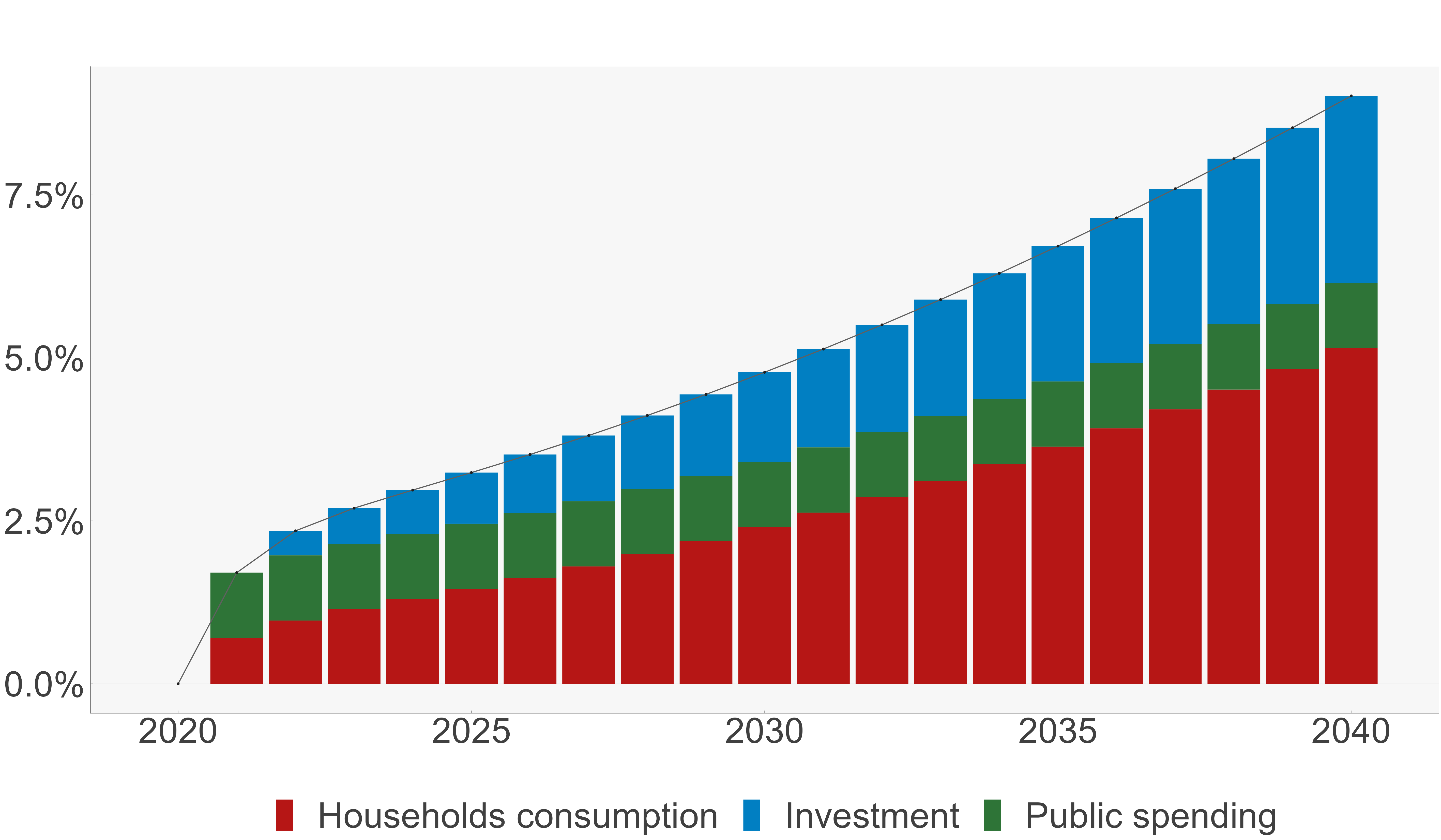
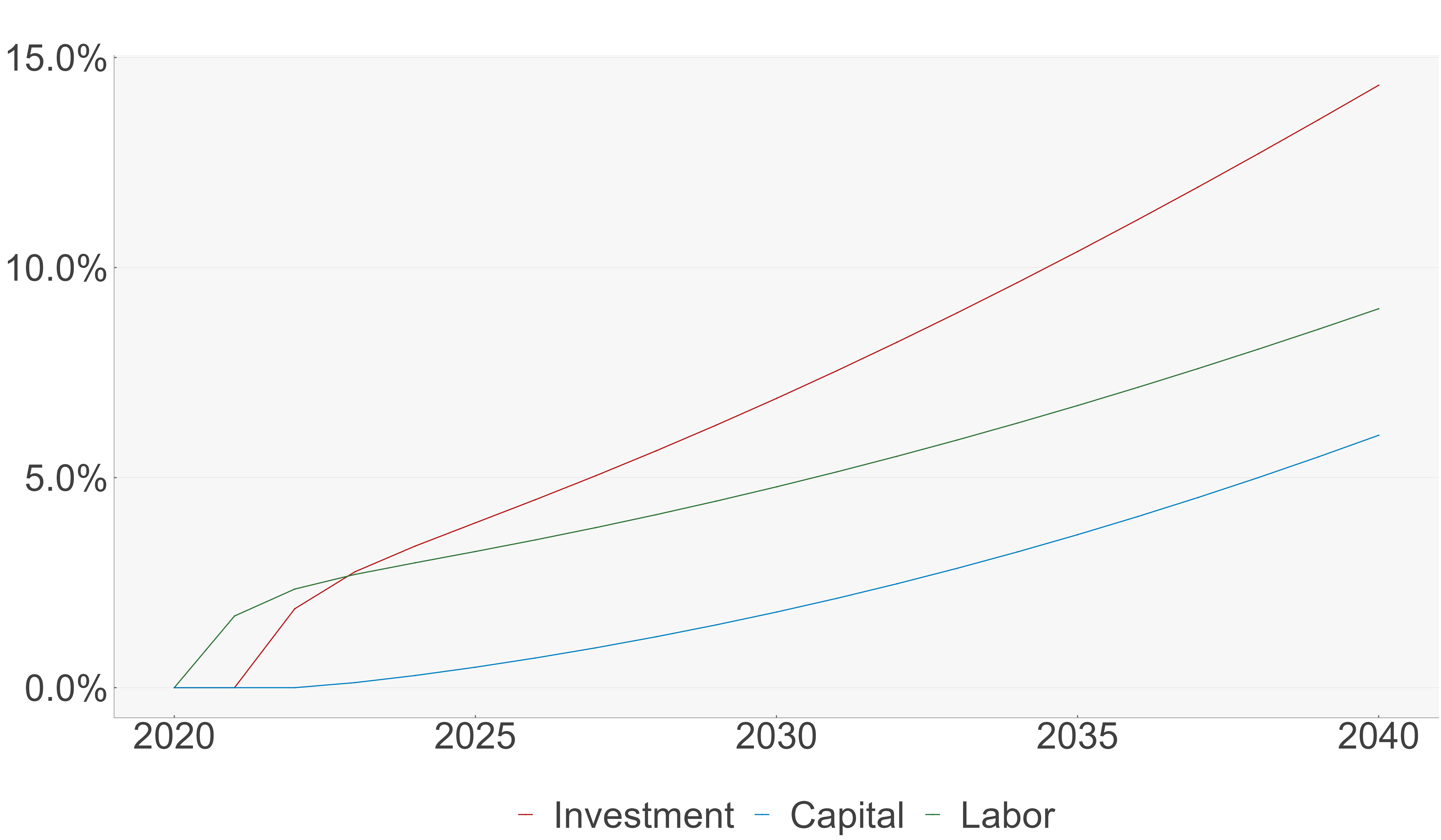
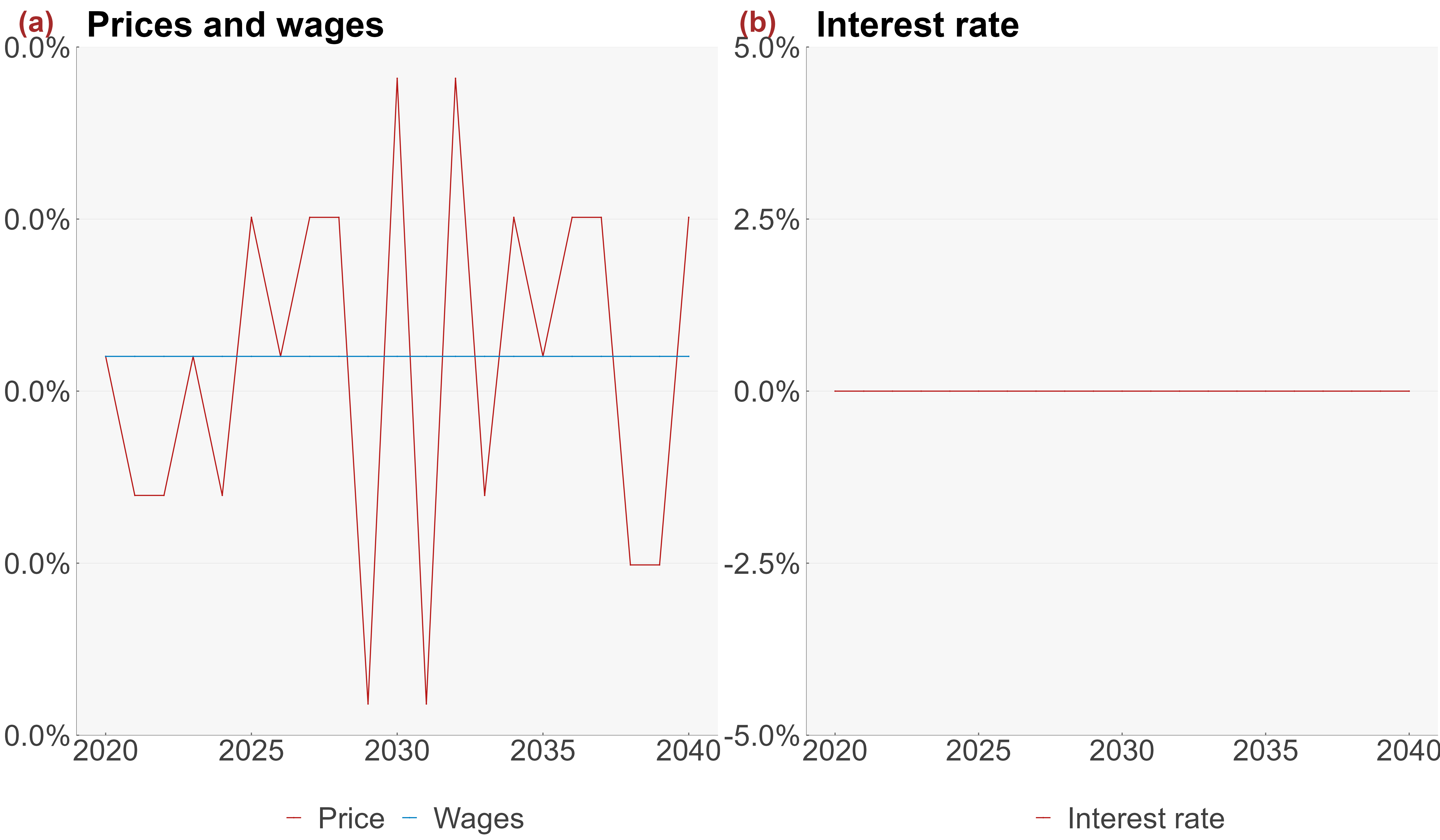
We present below some main results regarding the impact on public spending of one GDP point. We assume a long term steady state where the growth rate of volume and price variables is zero. This requires the assumptions that in the long term the growth rate of technical progress and of the population is zero. Increasing public spending result on the following effects: - Positive multiplier (Crowding in effect): the increase in public spending has an immediate positive effect on the economy (Figure 1), contrarily to the Walrasian model where the impact of an increase in public spending leads to a negative multiplier - The supply constraint is no more held: production is no more predetermined by labor and capital (implicit assumption of non used production) - As production increases, more factors are needed which increases demand for labor and capital (Figure 2). Increasing labor and capital rises production which increases consumption and investment - Prices, wages and interest rate remain constant (Figure 3)
Annexes
Endogenous variables’ equations
Production (GDP) \[Y = CH + I + G \tag{1}\]
Price \[p . Y = w . L + p . \left( \delta + r \right) . K^{n} \tag{2}\]
Households’consumption \[CH = \left( 1 - \sigma \right) . \frac{\left( w . L + p . r . K \right)}{p} \tag{3}\]
Labor demand \[L = \left( \frac{Y}{PROG^{L}} \right) . \left( \left( \varphi^{L} \right) ^ {\rho} \right) . \left( \frac{w}{\left( p . PROG^{L} \right)} \right) ^ {\left( -\rho \right)} \tag{4}\]
Capital demand (notional level from cost minimization assuming a CES function) \[K^{n} = \left( \frac{Y}{PROG^{K}} \right) . \left( \left( \varphi^{K} \right) ^ {\rho} \right) . \left( \frac{\left( \delta + r \right)}{PROG^{K}} \right) ^ {\left( -\rho \right)} \tag{5}\]
Capital (effective level from accumulation equation) \[\varDelta \left(K\right) = I_{t-1} - \delta . K_{t-1} \tag{6}\]
Investment \[\varDelta \left(\operatorname{log} I\right) = \varDelta \left(\operatorname{log} K^{n}_{t-1}\right) + alpha^{I,Kn} . \operatorname{log} \frac{K^{n}_{t-1}}{K_{t-1}} \tag{7}\]
Glossary of variables
| \(CH\) | Households’consumption | 3 |
| \(I\) | Investment | 7 |
| \(K\) | Capital (effective level from accumulation equation) | 6 |
| \(K^{n}\) | Capital demand (notional level from cost minimization assuming a CES function) | 5 |
| \(L\) | Labor demand | 4 |
| \(p\) | Price | 2 |
| \(Y\) | Production (GDP) | 1 |