ThreeME in detail
22 septembre 2023
Overview of the model
Production function and demand for production factors
Greenhouse gases emissions
ThreeME is a Computable General Equilibrium model (CGE). The general equilibrium is achieved by assuming that demand (consumption, investment, exports) determines supply (domestic production and imports). Supply defines in return demand through the incomes generated by the production factors (labor, capital, energy, material, land, etc.).
In the short and medium run, there can be situations of disequilibrium between notional (optimal) supply and the actual supply and of underutilization of the production capacity (in particular involuntary unemployment). In coherence with empirical evidence, it is assumed that prices and quantities are rigid in the short run and that they adjust slowly over time toward their optimal level.
ThreeME is an open source model and the full model code is available on Github:
For detailed description of the third version of the ThreeME model download the full documentation on the ThreeME website:
A neo-Keynesian CGE model
Main interactions
An important one is that demand determines supply. As a feed-back with eventually some lags, the supply affects the demand through several mechanisms:
The level of production determines the quantity of inputs used by the firms and thus the quantity of their intermediate consumptions and investment which are two components of the demand. It determines the level of employment as well and consequently the households final consumption.
Another effect of employment on demand goes through the wage setting via the unemployment rate which is also determined by the active population. Wages affect the household consumption because they are an important part of their income.
Prices and costs affect profits and therefore households’ consumption thought dividends and investment thought the sectors’ debts level.
Another canal is the monetary policy which is defined by a Taylor rule. The Central Bank determines the interest rate level based on inflation and unemployment. This has an effect on the demand via the negative effect of the real interest rate on consumption and investment.
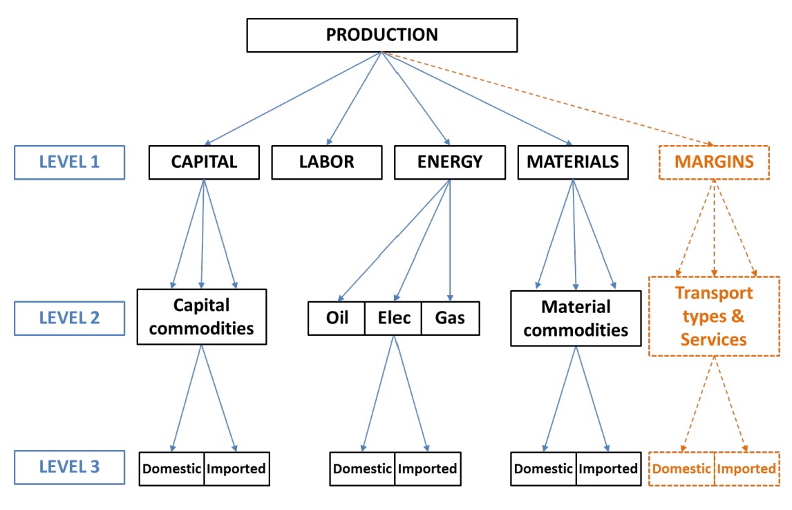
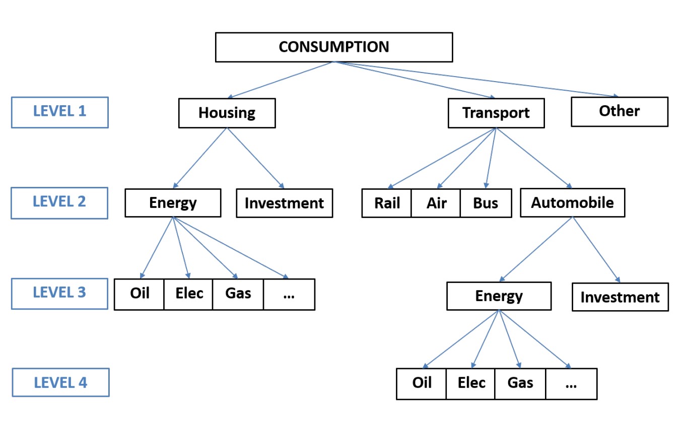
The dynamic of prices is the driver of the substitution mechanisms of the model. Importantly for the analysis of environmental and energy policies, the prices dynamics defines the substitutions between production factors (in particular between capital and energy) and the share of each energy and transport into (intermediate and final) consumptions.
Adjustment mechanisms
Production function and demand for production factors
Greenhouse gases emissions
ThreeME represents the functioning of the economy by taking into account explicitly the slow adjustment of prices and quantities (factors of production, consumption). In this neo-Keynesian framework, permanent or transitory underemployment equilibria are possible and supply is determined by demand.
ThreeME assumes that the actual levels of prices and quantities gradually adjust to their notional level. The notional level corresponds to the optimal (desired or target) level that the economic agent in question (the producer for prices and the demand for production factors, the household for consumption, the Central bank for the interest rate, etc.) would choose in the absence of adjustment constraints.
Formally, we assume that the adjustment process and expectations for prices and quantities are represented by the following equations:
\[\begin{equation}
\label{eq-efective_adjustement}
\small
\operatorname{log} X_{t} = \alpha^{{0},X} \; \operatorname{log} X^{n}_{t} + \left( 1 - \alpha^{{0},X} \right) \; \left( \operatorname{log} X_{t-1} + \varDelta \left(\operatorname{log} X^{e}_{t}\right) \right)
\end{equation}\]
\[\begin{equation}
\small
\begin{split}
\label{eq-expected_adjustement}
\varDelta \left(\operatorname{log} X^{e}_{t}\right) = \alpha^{{1},X} \; \varDelta \left(\operatorname{log} X^{e}_{t-1}\right) + \alpha^{{2},X}\; \varDelta \left(\operatorname{log} X_{t-1}\right)
+ \alpha^{{3},X} \; \varDelta \left(\operatorname{log} X^{n}_t\right) + \alpha^{{4},X} \; \varDelta \left(\operatorname{log} X_{t+1}\right)
\end{split}
\end{equation}\]
Where \(X_{t}\) is the effective value of a given variable, \(X^{n}_t\) is its notional level, \(X^{e}_t\) its expected (anticipated) value at period \(t\) and \(\alpha^{{i},X}\) are the adjustments parameters, with \(\alpha^{{1},X} + \alpha^{{2},X} + \alpha^{{3},X} + \alpha^{{4},X} = 1\).
Production function and demand for production factors
Production function and demand for production factors
Greenhouse gases emissions
![]()
Demand for production factors
The production costs minimization program leads to the following equations for the notional factors demand:
\[\begin{equation}
\small
\varDelta \left(\operatorname{log} F^{n}_{f, s}\right) = \varDelta \left(\operatorname{log} Y_{s}\right) - \varDelta \left(\operatorname{log} PROG_{f, s}\right) + \varDelta \left(SUBST^{F}_{f, s}\right)
\end{equation}\]
\[\begin{equation}
\tiny
\varDelta \left(SUBST^{F,n}_{f, s}\right) = \sum_{ff} -ES_{f, ff, s} \; \varphi_{ff, s, t-1} \; \varDelta \left(\operatorname{log} \frac{C_{f, s}}{PROG_{f, s}} - \operatorname{log} \frac{C_{ff, s}}{PROG_{ff, s}}\right)
\end{equation}\]
where
\[\begin{equation}
\small
\varphi_{f, s} = \frac{C_{f, s} \; F^{n}_{f, s}}{\sum_{ff} C_{ff, s} \; F^{n}_{ff, s}}
\end{equation}\]
with:
- The notional demand of input \(f\) (\(KLEM\)): \(F_{f,s}^n\)
- The elasticity of substitution between the pairs of inputs \(f\) and \(ff\): \(ES_{f,ff,s}\)
- The technical progress related to input \(f\): \(PROG_{f,s}\)
- The cost/price of input \(f\): \(C_{f,s}\)
- The level of production of the sector \(s\): \(Y_{s}\)
Demand for production factors
The production of each sector is defined by the following equations:
\[\begin{equation}
\small
Y_{c, s} = \varphi^{Y}_{c, s} \; YQ_{c}
\end{equation}\]
\[\begin{equation}
\small
Y = \sum_{s} Y_{s}
\end{equation}\]
where \(YQ_c\) is the aggregated domestic production of commodity \(c\). It is determined by the demand (intermediate and final consumption, investment, public spending, exports and stock variation). \(PhiY_{c, s}\) is then the share of commodity \(c\) produced by the sector \(s\) (with \(\sum_{s} phiY_{c,s} =1\)) and \(Y_s\) is the aggregated production of sector \(s\).
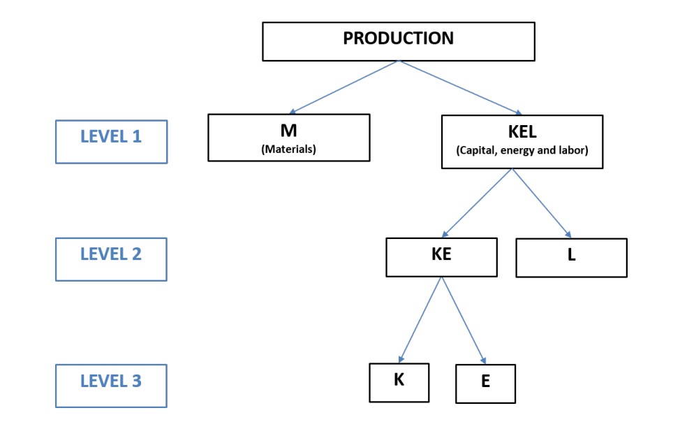
Nested CES production function
At the first level, material (M) can be substituted with the aggregate capital/energy/labor (KEL) with an ES of \(\sigma^{NEST^{MAT,KEL}}\) .
At the second level, the aggregate capital/energy (KE) is a substitute to labor (L) with an ES of \(\sigma^{NEST^{KE,L}}\).
At the third level, capital (K) can be substituted to energy (E) with an ES of \(\sigma^{NEST^{K,E}}\).
\[\begin{equation}
ES_{K, E, s} = \frac{\eta^{NEST^{K,E}}_{s}}{\left( 1 - \varphi_{MAT, s} - \varphi_{L, s} \right) - \frac{\eta^{NEST^{MAT,KEL}}_{s}}{\left( 1 - \varphi_{MAT, s} \right) - \eta^{NEST^{KE,L}}_{s} \; \frac{\varphi_{L, s}}{\frac{1 - \varphi_{MAT, s}}{1 - \varphi_{MAT, s} - \varphi_{L, s}}}}}
\end{equation}\]
\[\begin{equation}
ES_{K, L, s} = \frac{\eta^{NEST^{KE,L}}_{s} - \eta^{NEST^{MAT,KEL}}_{s} \; \varphi_{MAT, s}}{1 - \varphi_{MAT, s}}
\end{equation}\]
Nested CES production function: a scheme
![]()
Investment and capital
Investment in ThreeME depends on the anticipated production, on its past dynamic, on substitution phenomena and on a correction mechanism, which guaranties that companies reach their level of long-term notional capital stock. The stock of capital is deducted from the investment according to the standard capital accumulation equation:
\[\begin{equation}
\small
\begin{split}
\varDelta \left(\operatorname{log} IA_{s}\right) = \alpha^{IA,Ye}_{s} \; \varDelta \left(\operatorname{log} Y^{e}_{s}\right) + \alpha^{IA,IA1}_{s} \; \varDelta \left(\operatorname{log} IA_{s, t-1}\right) \\
+ \alpha^{IA,SUBST}_{s} \; \varDelta \left(SUBST^{F}_{K, s}\right) \\
+ \alpha^{IA,Kn}_{s} \; \left( \operatorname{log} F^{n}_{K, s, t-1} - \operatorname{log} F_{K, s, t-1} \right)
\end{split}
\end{equation}\]
\[\begin{equation}
\small
F_{K, s} = \left( 1 - \delta_{s} \right) \; F_{K, s, t-1} + IA_{s}
\end{equation}\]
Price setting
Production function and demand for production factors
Greenhouse gases emissions
The production price for each sector is set by applying a mark-up over the unit cost of production (which includes labor, capital, energy and other intermediate consumption costs):
\[\begin{equation}
\small
PY^{n}_{s} = CU^{n}_{s} \; \left( 1 + \mu_{s} \right)
\end{equation}\]
Where \(PY^n\) is the notional price, \(CU^n_s\) the unitary cost of production and \(\mu_{s}\) is the mark-up.
Notional mark-up of the sector \(s\): the default notional mark-up is a positive function of the capacity utilization ratio.
\[\begin{equation}
\small
\varDelta \left(\operatorname{log} \left(1 + \mu^{n}_{s}\right)\right) = \rho^{\mu,Y} . \varDelta \left(\operatorname{log} CUR_{s}\right)
\end{equation}\]
\[\begin{equation}
CUR_{s} = \frac{Y_{s}}{YCAP_{s}}
\end{equation}\]
\[\begin{equation}
\begin{split}
\varDelta \left(\operatorname{log} YCAP_{s}\right) = \sum_{f} \varphi_{f, s, t-1} \; \varDelta \left(\operatorname{log} \left(F_{f, s} \; PROG_{f, s}\right)\right)
+ \alpha^{YCAP,Y}_{s} \; \left( \operatorname{log} Y_{s, t-1} - \operatorname{log} \left(YCAP_{s, t-1} \; CUR_{s, t_0}\right) \right)
\end{split}
\end{equation}\]
Wage setting
Production function and demand for production factors
Greenhouse gases emissions
In ThreeME, we choose a general specification that includes the Phillips and Wage Setting (WS) curves. It assumes that the notional nominal wage (\(W^n_s\)) positively depends on the anticipated consumption price (\(P^e\)) and on the labor productivity (\(PROG^L_s\)), and negatively on the unemployment rate (\(UnR\)):
\[\begin{equation}
\small
\begin{split}
\varDelta \left(\operatorname{log} W^{n}_{s}\right) = \rho^{W,Cons}_{s} + \rho^{W,P}_{s} \; \varDelta \left(\operatorname{log} P\right) + \rho^{W,Pe}_{s} \; \varDelta \left(\operatorname{log} P^{e}\right) \\
+ \rho^{W,PROG}_{s} \; \varDelta \left(\operatorname{log} PROG^{L}_{s}\right) - \rho^{W,U}_{s} \; \left( UnR - DNAIRU \right) \\
- \rho^{W,DU}_{s} \; \varDelta \left(UnR\right) + \rho^{W,L}_{s} \; \varDelta \left(\operatorname{log} F_{L, s} - \operatorname{log} F_{L}\right)
\end{split}
\end{equation}\]
This relation can alternatively be identical, either to the Phillips curve, or to the WS curve depending on the value of the selected parameters (Heyer et al., 2007; Reynès, 2010).
Interest rate
Production function and demand for production factors
Greenhouse gases emissions
In the neo-Keynesian framework, it is standard to assume that the interest rate is set by the Central Bank (CB) according to a Taylor rule (Taylor, 1993). The real interest rate is a positive function of inflation and a negative function of unemployment rate (here used as a proxi of the output gap):
\[\begin{equation}
\small
\varDelta \left(R^{n}\right) = \rho^{Rn,P} . \varDelta \left(\frac{\varDelta \left(P\right)}{P_{t-1}}\right) - \rho^{Rn,UnR} . \varDelta \left(UnR\right)
\end{equation}\]
Households’ consumption
Production function and demand for production factors
Greenhouse gases emissions
We assume that the notional (optimal) aggregate households consumption corresponds to a share of their current income:
\[\begin{equation}
\small
CH^{n,VAL} = DISPINC^{AT,VAL} . \left( 1 - MPS^{n} \right)
\end{equation}\]
Where \(CH^{n,VAL}\) is the aggregate notional households final consumption expressed in value, \(DISPINC^{AT,VAL}\) is the households’ disposable income and \(MPS^n\) their notional marginal propensity to save, defined as follows:
\[\begin{equation}
\small
\varDelta \left(MPS^{n}\right) = \rho^{MPS,R} . \varDelta \left(R - \frac{\varDelta \left(P\right)}{P_{t-1}}\right) + \rho^{MPS,UnR} . \varDelta \left(UnR\right)
\end{equation}\]
Variant 1: LES utility function
\[\begin{equation}
\small
\left( CH^{n}_{c} - NCH_{c} \right) \; PCH_{c} = \varphi^{MCH}_{c} \; \left( CH^{n,VAL} - PNCH . NCH \right)
\end{equation}\]
\[\begin{equation}
\small
\varDelta \left(\operatorname{log} \varphi^{MCH}_{c}\right) = \left( 1 - \eta^{LESCES} \right) . \varDelta \left(\operatorname{log} \frac{PCH_{c}}{PCH^{CES}}\right)
\end{equation}\]
\[\begin{equation}
\small
PCH^{CES} = \left( \sum_{c} \varphi^{MCH}_{c, t_0} \; PCH_{c} ^ {\left( 1 - \eta^{LESCES} \right)} \right) ^ {\left( \frac{1}{\left( 1 - \eta^{LESCES} \right)} \right)}
\end{equation}\]
Variant 2: Nested utility function
![]()
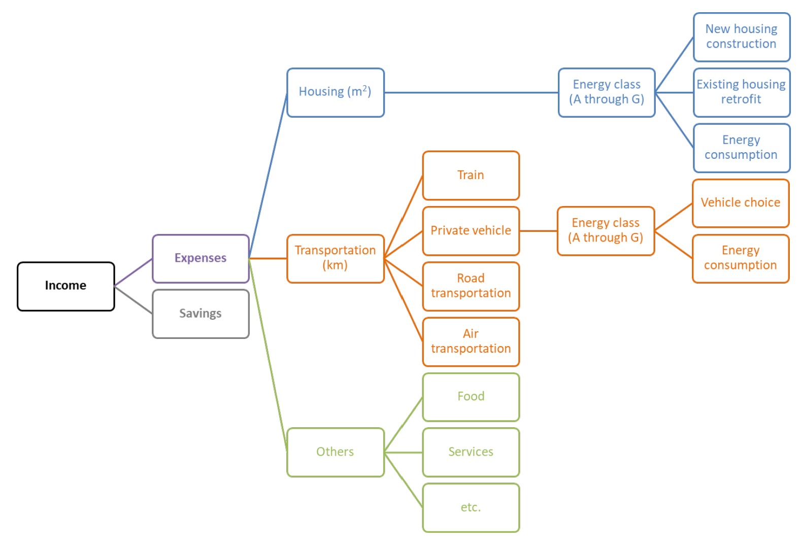
Variant 3: Hybrid approach
![]()
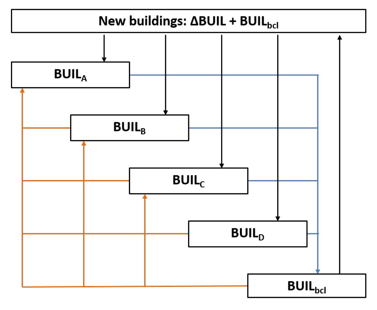
Building stock dynamic
\[\begin{equation}
\small
\begin{split}
\varDelta \left(BUIL_{ecl}\right) = NewBUIL_{ecl} + \sum_{ecl2} REHAB_{ecl2, ecl} \\
+ \sum_{ecl2} DEP^{BUIL}_{ecl2, ecl} - \left( \sum_{ecl2} REHAB_{ecl, ecl2} \right) \\
- \left( \sum_{bcl} DEP^{BUIL}_{ecl, bcl} \right)
\end{split}
\end{equation}\]
\[\begin{equation}
\small
REHAB_{ecl, ecl2} = \varphi^{REHAB}_{ecl, ecl2} \; \tau^{REHAB}_{ecl} \; BUIL_{ecl, t-1}
\end{equation}\]
\[\begin{equation}
\tiny
\tau^{REHAB,N}_{ecl} = \tau^{REHAB,MAX}_{ecl} + \frac{\tau^{REHAB,MIN}_{ecl} - \tau^{REHAB,MAX}_{ecl}}{1 + e^{\tau_{ecl} - \sigma_{ecl} \; Payback^{REHAB}_{ecl}}}
\end{equation}\]
\[\begin{equation}
\tiny
Payback^{REHAB}_{ecl} = \frac{UC^{K,REHAB}_{ecl} \; BUIL^{D}_{ecl} - UC^{K}_{ecl} \; BUIL^{D}_{ecl}}{UC^{E}_{ecl} - UC^{E,REHAB}_{ecl}}
\end{equation}\]
![]()
Foreign trade
Production function and demand for production factors
Greenhouse gases emissions
Foreign trade 1/2
-Exports are determined by the external demand addressed to domestic products and the ratio between the export and world prices:
\[\begin{equation}
\varDelta \left(\operatorname{log} X_{c}\right) = \varDelta \left(\operatorname{log} WD_{c}\right) + \varDelta \left(SUBST^{X}_{c}\right)
\end{equation}\]
\[\begin{equation}
\varDelta \left(SUBST^{X,n}_{c}\right) = -\eta^{X}_{c} \; \varDelta \left(\operatorname{log} PX_{c} - \operatorname{log} \left(EXR . PWD_{c}\right)\right)
\end{equation}\]
Where \(WD_{c}\) is the world demand, \(PWD_{c}\) its price. \(PX_{c}\) is the export price that depends on the production costs and which reflects the price-competitiveness of the domestic products. \(EXR\) is the exchange rate; \(\sigma^{X}_{c}\) is the price-elasticity (assumed constant).
Foreign trade 2/2
We assume imperfect substitution between domestic and imported goods (Armington, 1969). The demand for domestic and imported products is:
\[\begin{equation}
AD_{c} = \left( 1 - \varphi^{AM}_{c} \right) \; A_{c}
\end{equation}\]
\[\begin{equation}
\varphi^{AM}_{c} = \frac{1}{\left( 1 + \frac{AD_{c}}{AM_{c}, t_0} \; \operatorname{exp} SUBST^{AM}_{c} \right)}
\end{equation}\]
\[\begin{equation}
SUBST^{AM}_{c} = \alpha^{{6},AM}_{c} \; SUBST^{AM,n}_{c} + \left( 1 - \alpha^{{6},AM}_{c} \right) \; SUBST^{AM}_{c, t-1}
\end{equation}\]
\[\begin{equation}
\varDelta \left(SUBST^{AM,n}_{c}\right) = -\sigma^{AM}_{c} \; \varDelta \left(\operatorname{log} PAD_{c} - \operatorname{log} PAM_{c}\right)
\end{equation}\]
\[\begin{equation}
AM_{c} = \varphi^{AM}_{c} \; A_{c}
\end{equation}\]
Government
Production function and demand for production factors
Greenhouse gases emissions
Resources
According to the national accounts, public administrations generally refer to the central and regional government services and social security administration. In ThreeME, we have aggregated these three components in order to focus on transfers between public administrations, household and sectors.
These transfers are accounted for in the government’s resources \(INC^{G,VAL}\) and expenditures \(SPEND^{G,VAL}\):
\[\begin{equation}
\begin{split}
INC^{G,VAL} = PNTAXC . NTAXC + NTAXS^{VAL} + INC^{SOC,TAX,VAL} + PRSC . RSC + PROP^{INC,G,VAL}
\end{split}
\end{equation}\]
with:
- The aggregate net taxes on commodity \(c\) expressed in value: \(PNTAXC.NTAXC\)
- The aggregate net taxes on production of sectors expressed in value: \(NTAXS^VAL\)
- The income and social taxes expressed in value: \(INS^{SOC,TAX,VAL}\)
- The aggregate employers’ social security contribution paid by sector: \(PRSC.RSC\)
- The property income of the Government expressed in value: \(PROP^{INC,G,VAL}\)
Spendings
\[\begin{equation}
\begin{split}
SPEND^{G,VAL} = PG . G + SOC^{BENF,VAL} + DEBT^{G,VAL}_{t-1} \; \left( \varphi^{RD^{G}}_{t-1} + r^{DEBT,G}_{t-1} \right)
\end{split}
\end{equation}\]
with:
-The government final consumption: \(PG.G\)
-The Social benefits expressed in value: \(SOC^{BENF,VAL}\)
-The interest paid by the government on its debt plus the share of debt reimbursed every year: \[DEBT^{G,VAL}_{t-1}\left(\varphi^{RD^G}_{t-1} + r^{DEBT,G}_{t-1}\right)\]
Greenhouse gases emissions
Production function and demand for production factors
Greenhouse gases emissions
Concepts and approach
The modeling of the demand for fossil energy in ThreeME is detailed by economic agent and by sector for each energy source (coal, oil and gas). This allows for a precise estimation of the variation in the national greenhouse gases (\(GHG\)) emissions.
The calculation of emissions level consists in multiplying the fossil energy demand by the corresponding emission coefficients. These coefficients are specific for each gas, each economic actor, each sector and each energy sources depending on their carbon intensity.
Emissions accounting
-Emissions of the greenhouse gas \(ghg\) related to the intermediary consumption of commodity \(c\) by sector \(s\)
\[\begin{equation}
\small
\varDelta \left(\operatorname{log} EMS^{CI}_{ghg, c, s}\right) = \varDelta \left(\operatorname{log} \left(CI_{c, s} \; IEMS^{CI}_{ghg, c, s}\right)\right)
\end{equation}\]
where \(IEMS^{CI}_{ghg, c, s}\) is the corresponding emission intensity calibrated to 1 in the base year. It may change over time because of the increase of the share of biofuels.
-Emissions of the greenhouse gas \(ghg\) related to the household consumption \(c\)
\[\begin{equation}
\small
\varDelta \left(\operatorname{log} EMS^{CH}_{ghg, c}\right) = \varDelta \left(\operatorname{log} \left(CH_{c} \; IEMS^{CH}_{ghg, c}\right)\right)
\end{equation}\]
-Emissions of the greenhouse gas \(ghg\) related to the final production of sector \(s\)
\[\begin{equation}
\small
\varDelta \left(\operatorname{log} EMS^{Y}_{ghg, s}\right) = \varDelta \left(\operatorname{log} \left(Y_{s} \; IEMS^{Y}_{ghg, s}\right)\right)
\end{equation}\]
\(CO_2\) emissions from decarbonation during the production process for the non mineral metallic products, as the glass or ceramic sectors, is assumed proportional to the quantity of intermediate raw material used in the production process:
\[\begin{equation}
\small
\varDelta \left(\operatorname{log} EMS^{MAT}_{ghg, s}\right) = \varDelta \left(\operatorname{log} \left(F_{MAT, s} \; IEMS^{MAT}_{ghg, s}\right)\right)
\end{equation}\]
Energy balance
Production function and demand for production factors
Greenhouse gases emissions
Energy balance versus economic equilibrium
The energy module of ThreeME is based on a reformulation of the energy balance into meaningful economic concepts. The energy balance published by Eurostat uses the following definition for energy supply:
Total Primary Energy Supply (TPES) = Primary production + Imports - Exports + Change in stock (energy balance definition)
Energy intermediary consumptions as defined in the national accounts correspond to three different concepts in the energy balance:
Energy transformation input
Energy sector own use excluding the auto-consumptions.
Final consumption of non-energy sectors (final in the sense of the energy balance).
Energy accounting
In order to facilitate the link between the energy balance in physical units to the national accounts equilibrium defined in ThreeME, we have to rewrite the energy balance consistently. For this, we first need to make a distinction between the gross supply and the net supply of an energy commodity. The gross supply includes the domestic and imported primary and secondary production (as defined in the energy balance):
Gross supply = Primary production + Energy transformation output (secondary production) + Imports
The gross supply is not relevant economically for the end user because it includes distribution losses and auto-consumption. What is relevant for the end user is what she actually purchases, i.e. the domestic and imported supply net from distribution losses and auto-consumption:
Net supply = Domestic net production + Imported net production = Gross supply - Distribution losses - Auto-consumption
With this definition, we can rewrite the energy balance in an economically consistent way where the net supply of an energy commodity should be equal to its end use:
Net supply = Energy transformation input + Energy sector own use (excluding auto-consumption) + Final consumption + Exports + Change in stock (national account definition)