Introduction
In CGEM models supply equals demand at any time in all markets, what we call an equilibrium. There are several ways (closure) to guarantee this equilibrium. The most common and rather contrasting model closures are:
- The Walrasian closure
- The Keynesian closure
When modelers decide which variables are exogenous and which are endogenous, they define a model closure Burfisher (2021). Endogenous variables are defined inside the model, as a result of the model simulation with one equation for each endogenous variable. Examples of endogenous variables may be : production, consumption, prices, wages. Exogenous variables are defined outside the model with no equation in the model defining this variable. Examples of exogenous variables may include :population or the price of imports. Parameters are exogenous variable that are generally constant, such as the tax rate or elasticities. The quations of a model will solve for the endogenous variables, given the exogenous variables and parameters. A change in one or more exogenous variable or parameter will lead to adjustments in the endogenous variables so to solve the system of equations again. These solved values of all endogenous variables constitute the outcome of the model.
In this chapter and in the next one, we investigate the impact of the choice of a model closure on the long term and dynamic properties of CGEM in particular in terms of the multiplier of public expenditures. This chapter discusses the Walrasian closure and simulates the impact of an increase in public spending in this framework. The Keynesian closure will be discussed in the next chapter.
The selection of exogenous accounts, typically some combination of the government, savings-investment, and rest-of-the-world accounts, determines the macro ‘closure’ of the model Robinson (2006). The impact of the closure has been abundantly treated in the literature since the seminal work of Sen (1963) in a static framework. Sen showed that the necessary ex-post equality between investment and savings could not be satisfied if the following four conditions are simultaneously are met: (i) full employment of labor, (ii) factors paid at their marginal productivity, (iii) household consumption as a function of real income only, and (iv) a fixed amount of investment Dewatripont et Michel (1987). The choice of the closure rule and the condition to relax to achieve equilibrium has been subject of debate in the literature that has not reached consensual conclusions on this topic Dewatripont et Michel (1987). The appropriate choice between the different macro closures in the classic CGE model depends on the context of the analysis Robinson (2006). For example, if the model is for a single period and the purpose is to explore the equilibrium welfare changes of alternative policies, the preferred alternative may be a variant of the ‘Johansen’ closure that combines fixed foreign savings, fixed real investment, and fixed real government spending. However, if the analysis aims at capturing the effects of an exogenous shock or policy change , it is generally preferable to impose a more realistic closure that allowing the adjustment to macro shocks to be spread more evenly across the different components of consumption and investment Robinson (2006).
Since the seminal work of Sen (1963), the contributions of macroeconomics have opened the debate on several issues, including for example trade balance adjustments and the modeling of saving and accumulation behaviors especially the balance between investment and savings, the modeling of the interest rate using a Taylor rule and the modeling of household interest rate. Studies following the seminal work of Sen (1963) generally find that an exogenous increase in public expenditures leads to a decrease in production and therefore to a negative multiplier with a Walrasian (also referred as neo-classical) whereas it leads to a positive multiplier with a Keynesian closure (for a literature revue see e.g. Robinson (2006) or Zalai et Révész (2016)).
Dewatripont et Michel (1987) adresses the issue of model ‘closure’ by focusing on the implicit behavioral assumption leading to the existence of the closure problem using a simple temporary equilibrium to make explicit the micro-economic behavior. The paper discusses the implications of this analysis for the construction of a theoretical framework for fully dynamic general equilibrium models. In fully dynamic models, the equilibrium of each period depends both on current stock variables and on expectations of future states of the economy Dewatripont et Michel (1987). On the contrary, multi-period CGE models of the type described by Dervis et al. (1982) or surveyed by Shoven et Whalley (1984) rely typically on a sequence of static one-period solutions. In addition, dynamic macro CGE model are much richer, including assets, interest rates, inflation, expectations, and other features drawn from modern macro theory Robinson (2006).
Walrasian CGEM are static models that generally assume that the capital supply is fixed during the simulation period. Whereas certain Walrasian CGEM assume that the evolution of the capital stock as fully exogenous, a preferred approach in the literature is to assume that the change in capital stock over time is defined by a recursive dynamic Dixon et al. (2013).
Contrary to the literature that considers the static case where capital accumulation is not considered and investment has no impact on the capital stock and therefore on production capacity, we propose simulations based on a dynamic model including an equation for capital accumulation and where investment is endogenous (both in the Walrasian and in the Keynesian closures).
Section 2 presents the model’s Walrasian closure while (Section 3) displays the simulation results.
The Walrasian model closure
The Walrasian closure is based on the assumption of market clearing price: prices adjust to equilibrate supply and demand, which is known as an equilibrium theory. In other words, in Walrasian closure perfect flexibility of prices and quantities (production factors, consumption…) ensures the equilibrium between supply and demand. When an exogenous shock decreases the supply of a commodity, its price goes up, thereby stimulating additional supply and depressing demand, so that supply and demand stay always equal. The underlying assumptions of the Walrasian closure assume that labor supply is an exogenous variable (wage flexibility ensures full employment) and that the price is an exogenous variable defined as the numéraire: \(p_t\) =1 for all t.
The basic Walrasian framework is made of 7 endogenous variables and 7 equations. As said previously, the price equation Équation 7 defines the price as numéraire (equal to 1), and is set therefore as an exogenous variable. The model could equivalently be written as a set of 6 equations with 6 endogenous variables.
Wage
In the Walrasian closure, labor is exogenous. Therefore, the equation of labor demand (3.4) defined in Chapter 1 does not determine labor but wage. Wages adjust to clear markets.
The wage equation Équation 4 derives from cost minimization assuming a CES function and is obtained by adding and subtracting \(w_t\) on both sides of labor demand equation. This mathematical rearrangement does not change the results.
\[w + L = \left( \left( \frac{Y}{PROG^{L}} \right) . \left( \left( \varphi^{L} \right) ^ {\rho} \right) . \left( \frac{w}{\left( p . PROG^{L} \right)} \right) ^ {\left( -\rho \right)} \right) + w\]
Capital
The equation that determines capital Équation 6 is the one of capital accumulation (3.6) defined in Chapter 1. The change in capital stock, which, given an initial capital stock, will define the following capital stocks.
\[\varDelta \left(K\right) = I_{t-1} - \delta . K_{t-1}\]
Production
The price being set at one (numéraire), the equation of price (3.2) defined in Chapter 1 determines production in the Walrasian model
\[Y . p = w . L + p . \left( \delta + r \right) . K\]
Note that combining the wage equation Équation 4 and the interest rate equation Équation 5 in the production Équation 2 equation provides an alternative form of equation Équation 2,which is exactly the CES production function (see the proof below) :
\[Y = [\phi_L.(L.PROG^L)^{\frac{\rho-1}{\rho}} + \phi_K.(K.PROG^K)^{\frac{\rho-1}{\rho}}]^{\frac{\rho}{\rho-1}}\]
Proof. \[ L = \frac{Y}{PROG^{L}}. (\phi_L)^{\rho}.(\frac{w}{p.PROG^{L}})^{-\rho}\\ \frac{L}{\frac{Y}{PROG^{L}}.(\phi_L)^{\rho}}= (\frac{w}{p.PROG^{L}})^{-\rho}\\ \frac{w}{p.PROG^{L}}= \phi_L.(\frac{Y}{PROG^{L}.L})^{\frac{1}{\rho}}\\ K = \frac{Y}{PROG^{K}}. (\phi_K)^{\rho}.(\frac{\delta +r}{PROG^{K}})^{-\rho}\\ \frac{K}{\frac{Y}{PROG^{K}}.(\phi_K)^{\rho}}= (\frac{\delta + r}{PROG^{K}})^{-\rho}\\ \frac{\delta + r}{PROG^{K}}= \phi_K.(\frac{Y}{PROG^{K}.K})^{\frac{1}{\rho}}\\ p.Y= w.L+ p.(\delta+r).K\\ Y= \frac{w}{p}.L+ (\delta+r).K\\ Y= \phi_L.(PROG^{L})^{\frac{\rho-1}{\rho}}.Y^{\frac{1}{\rho}}.\frac{L}{L^{\frac{1}{\rho}}} + \phi_K.(PROG^{K})^{\frac{\rho-1}{\rho}}.Y^{\frac{1}{\rho}}.\frac{K}{K^{\frac{1}{\rho}}}\\ \frac{Y}{Y^{\frac{1}{\rho}}}=\phi_L.(PROG^{L})^{\frac{\rho-1}{\rho}}.L^{\frac{\rho-1}{\rho}} + \phi_K.(PROG^{K})^{\frac{\rho-1}{\rho}}.K^{\frac{\rho-1}{\rho}}\\ Y=[\phi_L.(L.PROG^{L})^{\frac{\rho-1}{\rho}} + \phi_K.(K.PROG^{K})^{\frac{\rho-1}{\rho}}]^{\frac{\rho}{\rho-1}}\\ \]
Investment
In Chapter 1, the equation of production (3.1) defines production (\(Y\)) as the endogenous variable.
In the Walrasian closure, we use this equation to determine investment. The later is defined endogenously as the difference between production and (private and public) consumption Équation 1. Therefore, savings define investment.
\[I = Y - CH - G\]
Interest rate
In the Walrasian closure, capital is exogenous. The equation of capital demand (3.5) defined in Chapter 1 does not determine capital but interest rate. Interest rates adjust to clear markets. The interest rate equation Équation 5 derives from cost minimization assuming a CES function and is obtained by adding and subtracting \(r_t\) on both sides of capital demand equation. This mathematical rearrangement does not change the results.
\[r + K = \left( \left( \frac{Y}{PROG^{K}} \right) . \left( \left( \varphi^{K} \right) ^ {\rho} \right) . \left( \frac{\left( \delta + r \right)}{PROG^{K}} \right) ^ {\left( -\rho \right)} \right) + r\]
Household’s consumption
We consider that households supply labor and capital, for which they get their income (\(w.L + p.r.k\)) . We assume that households wish to use a fixed share of their total income for consumption. The equation determining household’s consumption Équation 3 is the same as the one defined in Chapter 1.
\[CH = \left( 1 - \sigma \right) . \frac{\left( w . L + p . r . K \right)}{p}\]
Simulation results
We present below some main results regarding the impact on public spending of one GDP point. We assume a long term steady state where the growth rate of volume and price variables is zero. This requires the assumptions that in the long term the growth rate of technical progress and of the population is zero. Increasing public spending results on the following effects:
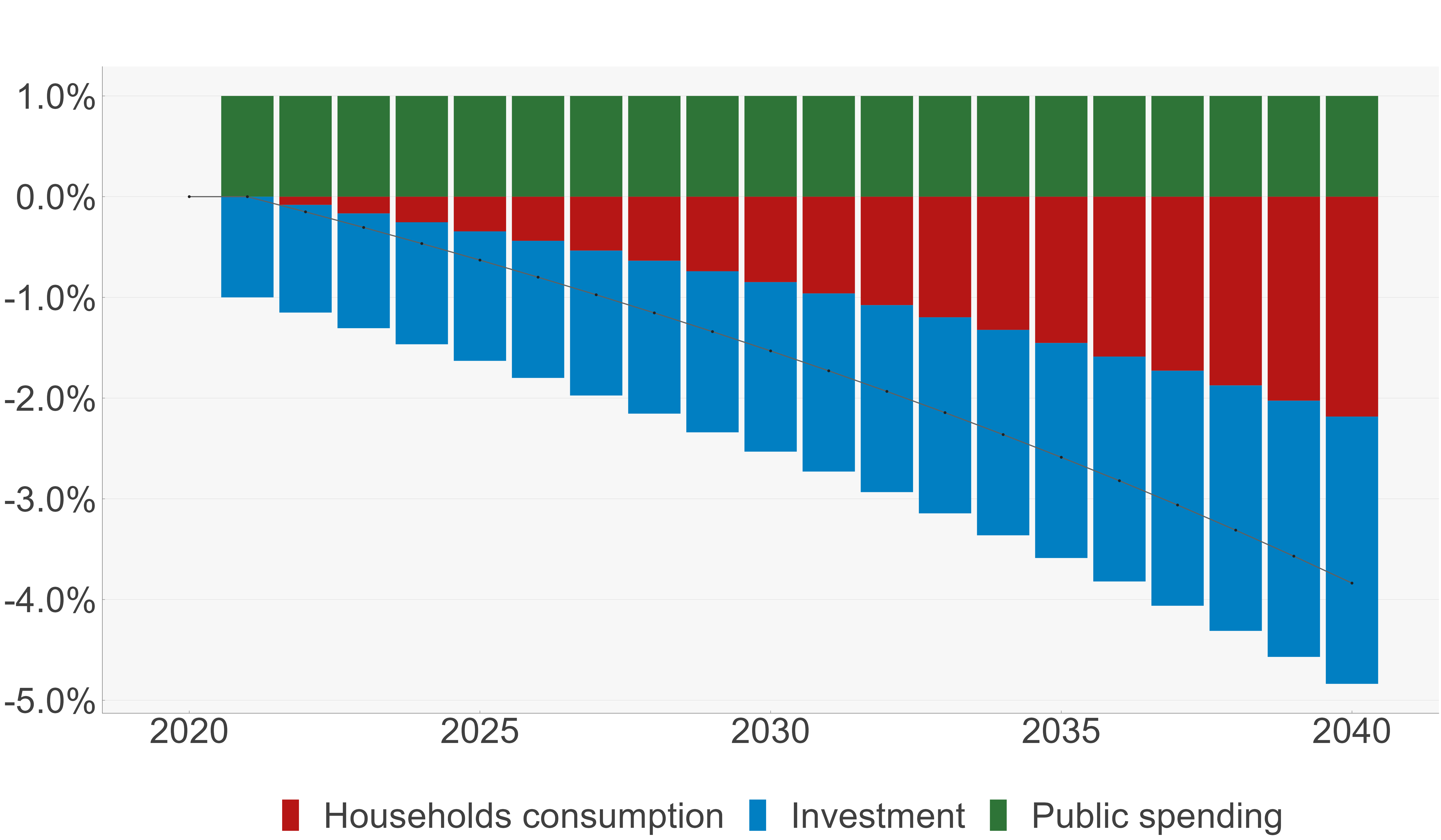
- Negative multiplier due to crowding out effect: rising public spending leads to a decrease of private expenditure (consumption and investment). Production is determined by the level of capital and labor in a given. There is no spare production capacity. Increasing public spending is only possible when diminishing investment and household’s consumption. (Figure 1)
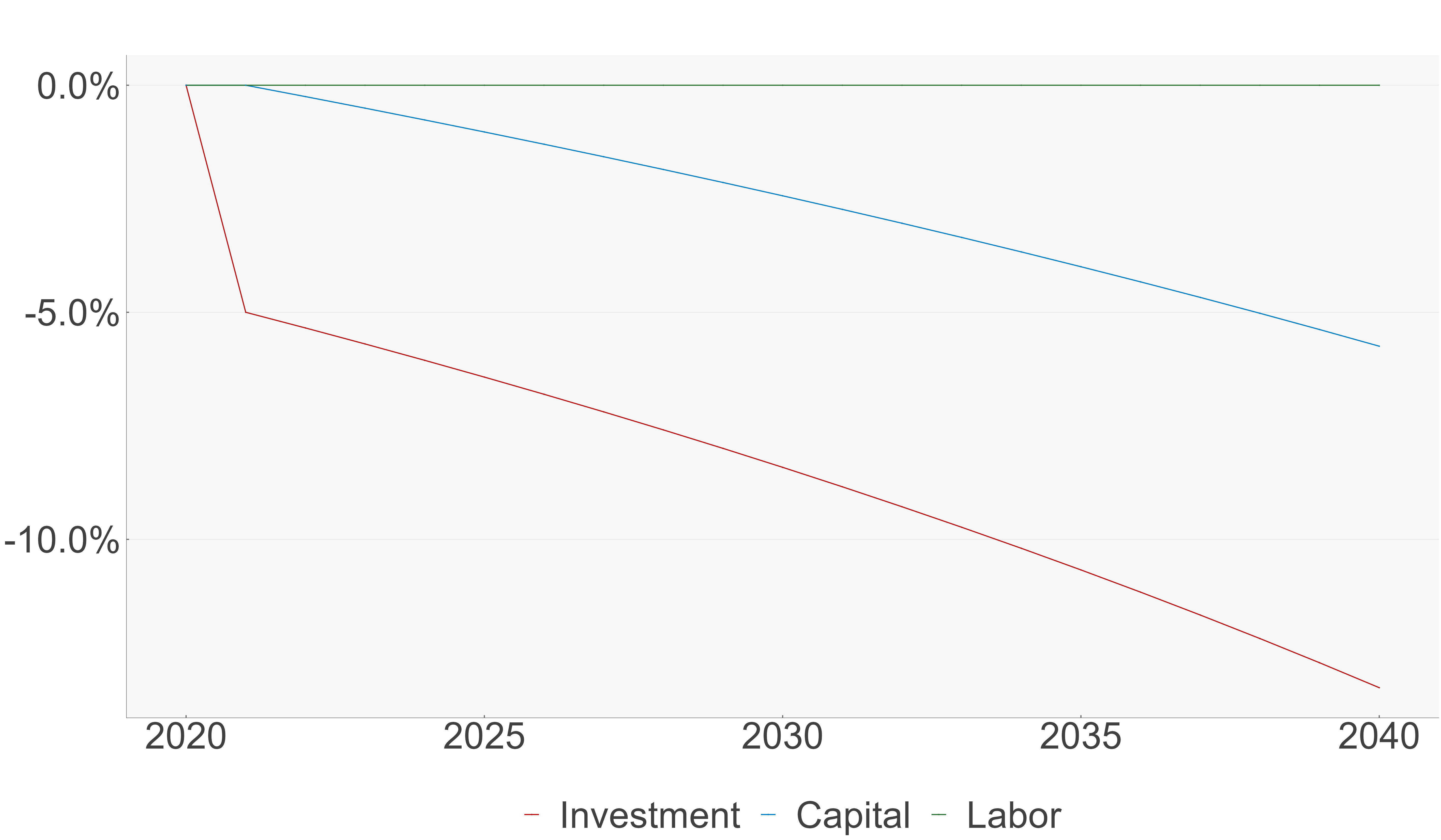
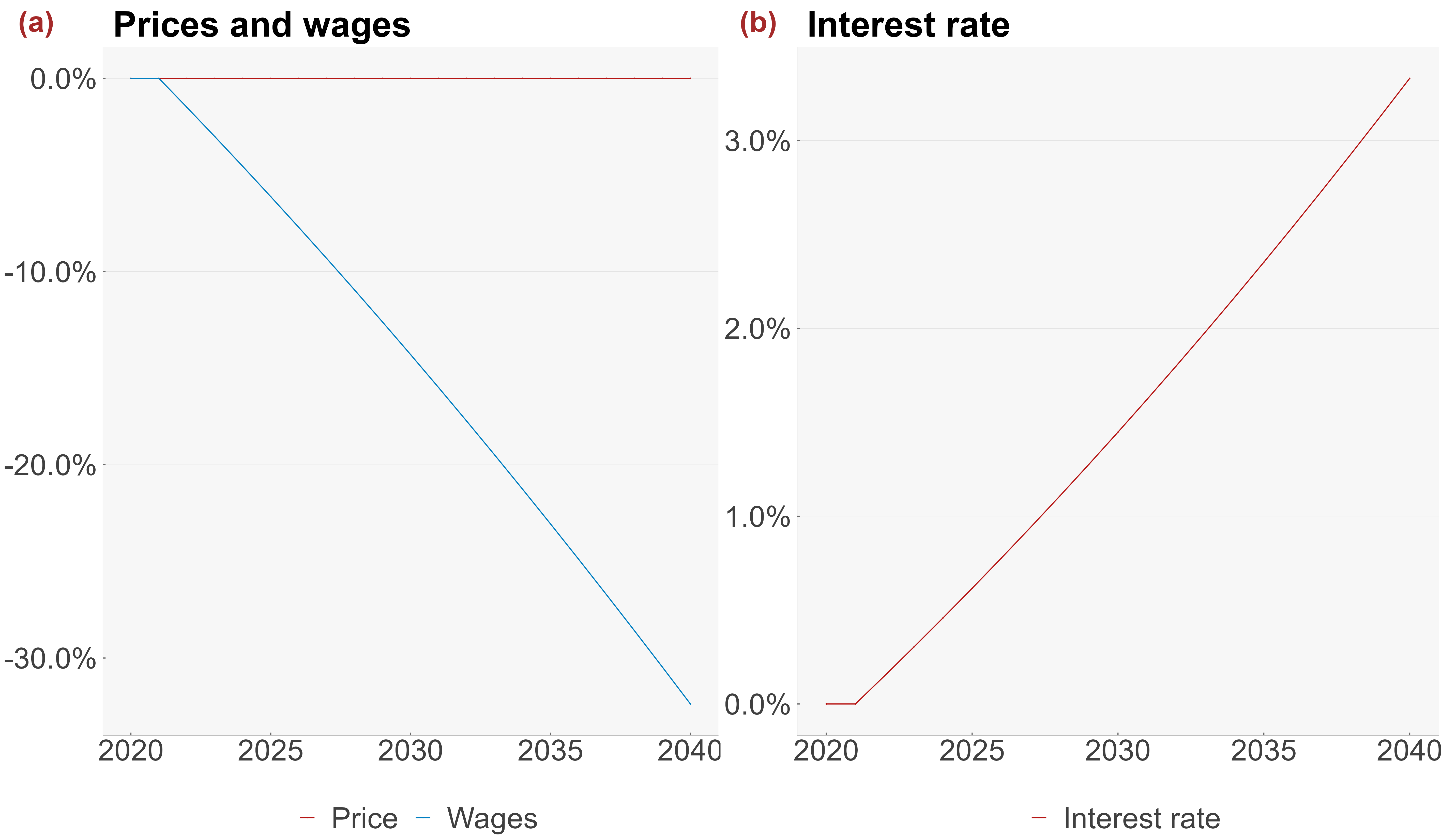
- Decreasing investment reduces the future capital stock capital (Figure 2), decreasing the interest rate (Figure 3). As capital decreases, production also decreases in the following period.
- As production decreases, wages decrease to keep full employment, which decrease further households’ income and consumption (Figure 3).
In this simple Walrasian model, an increase in public spending leads to a vicious negative cycle where public expenditure crowd-out private expenditure. The effect cumulative over time because of the decrease in the capital stock that reduce production over time.
Annexes
Endogenous variables’ equations
Investement \[I = Y - CH - G \tag{1}\]
Production (GDP) \[Y . p = w . L + p . \left( \delta + r \right) . K \tag{2}\]
Households’consumption \[CH = \left( 1 - \sigma \right) . \frac{\left( w . L + p . r . K \right)}{p} \tag{3}\]
Wage (from cost minimization assuming a CES function) \[w + L = \left( \left( \frac{Y}{PROG^{L}} \right) . \left( \left( \varphi^{L} \right) ^ {\rho} \right) . \left( \frac{w}{\left( p . PROG^{L} \right)} \right) ^ {\left( -\rho \right)} \right) + w \tag{4}\]
Interest rate (from cost minimization assuming a CES function) \[r + K = \left( \left( \frac{Y}{PROG^{K}} \right) . \left( \left( \varphi^{K} \right) ^ {\rho} \right) . \left( \frac{\left( \delta + r \right)}{PROG^{K}} \right) ^ {\left( -\rho \right)} \right) + r \tag{5}\]
Capital (from accumulation equation) \[\varDelta \left(K\right) = I_{t-1} - \delta . K_{t-1} \tag{6}\]
Price \[p = 1 \tag{7}\]
Glossary of variables
| \(CH\) | Households’consumption | 3 |
| \(I\) | Investement | 1 |
| \(K\) | Capital (from accumulation equation) | 6 |
| \(p\) | Price | 7 |
| \(r\) | Interest rate (from cost minimization assuming a CES function) | 5 |
| \(w\) | Wage (from cost minimization assuming a CES function) | 4 |
| \(Y\) | Production (GDP) | 2 |