Chapter 1: Introduction to CGE model
1 Introduction
Computable General Equilibrium (CGE) models have been widely used in the literature to simulate the impact of policies or external shocks on the economy.1 They are generally calibrated on actual data for potentially various geographical context (e.g. country, region) or sectoral detail. Allowing for a large range of concrete application, they are also referred to as Applied General Equilibrium models.
1 For a comparison of different types of CGEM see Dixon et Jorgenson (2012).
« Computable » refer to a numerical calculation whose objective is to simulate the evolution of key economics variables (such as GDP, consumption, prices, etc.) under the influence of a given context or policies.
The notion of « general equilibrium » relates to a state where supply is equal to demand in all markets. CGE models ambition to take into account the interaction and feedbacks between supply and demand as schematized in graphique 1. Demand (consumption, investment, exports) defines supply (domestic production and imports). Supply defines in return demand through the incomes generated by the production factors (labor, capital, energy, material, land, etc.).
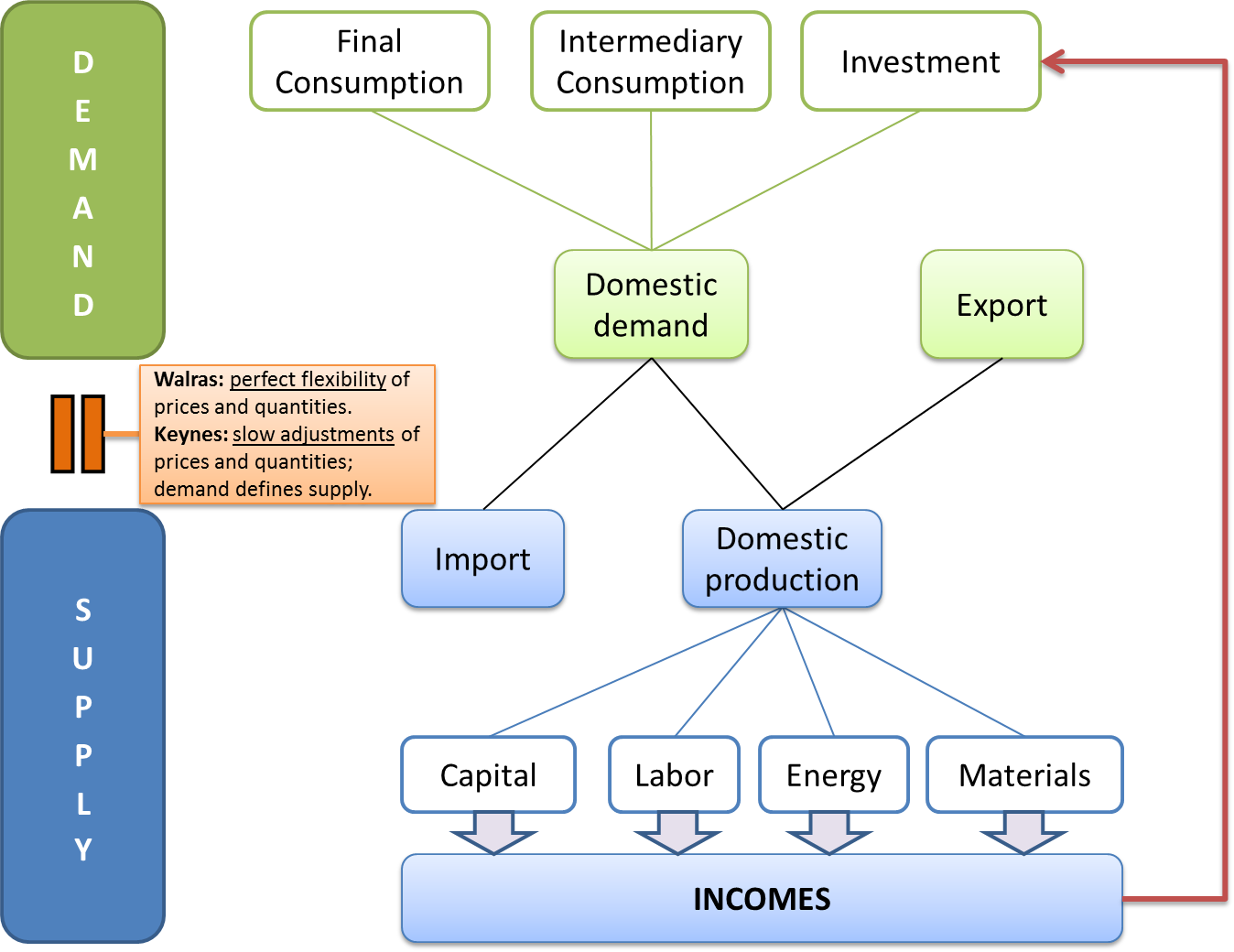
The very existence of a general equilibrium but also the concrete economic mechanisms allowing to reach such a state have led to one of the most important controversy in economics. This controversy has not been settled yet since there are still two main approaches used in the literature to ensure the general equilibrium. In Walrasian models, the equilibrium force is the price system. Perfect flexibility of prices and quantities (production factors, consumption, etc.) ensures the instantaneous equilibrium between supply and demand. For instance, when an exogenous shock decreases the supply of a commodity, its price tends to go up, thereby stimulating additional supply and depressing demand, until supply and demand are equal again. Arrow et Debreu (1954) demonstrate the conditions under which such an equilibrium exists.2 This equilibrium mechanism does not only operate on the product markets. Depending on the closures retained (see e.g. Shoven et Whalley (1992)), it may also apply on the production factors markets (labour, capital), on the saving market (savings equal investments) and on the foreign exchange markets (imports equal exports). Walrasian type of CGE models are often static: after a shock a new equilibrium (system of prices and quantities) is found within the period of simulation. However some Walrasian CGE models introduce a recursive dynamic where the past savings define next year capital stocks.
2 They demonstrate that the Walrasian equilibrium is a Nash equilibrium Nash (1950),Nash (1953) if agents are perfectly rational, if they do not commit anticipation errors, if the production functions do not show increasing returns to scale, and if the utility functions satisfy the standard properties of continuity, non-saturation and strict convexity of their isoquants. Additional more technical properties are also required (see e.g. Hahn (1982)).
The second approach is the one assumed in Keynesian models. In these models, prices do not clear the markets and market « imperfections » (e.g. involuntary unemployment) are taken into account. They assume that prices and quantities are rigid (at least) in the short run and that they adjust slowly over time toward their optimal level. The general equilibrium is achieved by assuming that demand determines supply. In the short and medium run, there can be situations of disequilibrium between notional (optimal) supply and the actual supply and of underutilization of the production capacity (in particular involuntary unemployment).
In the next two chapters, we shall see that Walrasian and Keynesian models can have radically different properties in terms of economic results and conclusion. Interestingly, they also rest on common foundations, in particular regarding the underlying rational microeconomic behaviors. One of the objective that this introduction to CGE models it to put this forward since we believe that understanding this similarities if key to for understanding the opposition between Walrasian and Keynesian models.
section 2 provides the key microeconomic foundation of CGE models. It provides the derivation of each equations of the model. The last three sections summarise the list of equations and variables that will be used to specify and simulate a simple Walrasian CGE model (Chapter 2) and simple Keynesian CGE model (Chapter 3). To avoid repetition, the Glossary section at the end of this chapter provides a table with the definition of the variables and parameters used in the model’s equations.
2 Micro-economic foundation
Computable General Equilibrium (CGE) models have behavioral and identity equations. Behavioral equations describe the economic behavior of producers, consumers, and other agents in the model based on microeconomic theory and economic rationality. Identity equations define a variable according to a definition as a mathematical function (sum, product, etc.) of other variables. Identity equations therefore hold true by definition. If the value of any one of the variables in the identity equation changes, then one or more of the other variables must also change in order to maintain the equivalence Burfisher (2021). Some of the equations do not need an explicit derivation as they can be considered simple accounting equations (e.g. GDP).
2.1 Behavior equations
2.1.1 Prices
We assume oligopolistic competition à la Cournot where each producer defines its price in order to maximise its profit considering the price of the other producers as given (Nash equilibrium). Assuming a demand function that relates negatively the demand addressed to the firm to its price, the optimal price can be defined according the following maximization program:
\[max_y {\Pi (y) = p(y).y - c(y)}\]
where \(y\) is the production or the demand addressed to the company, \(\Pi(y)\) is the profit of the company, \(p(y)\) its price and \(c(y)\) the production cost. We assume further that \(p'(y)<0, c'(y)> 0 \ and \ c''(y)> 0\).
The result of the program maximisation defines the long term optimum price that is equal to markup over production:
\[p(y) = [1 + m^{up}]. c'(y)\]
where \(m^{up}= \frac{1}{\epsilon -1}\) is the markup over the production costs. \(\epsilon\) is the (absolute) price elasticity of demand.
Proof. The first order condition is:
\[ \dfrac{\partial \Pi (y)}{\partial y} = 0 \Longleftrightarrow p'(y).y + p(y)- c'(y)= 0 \Longleftrightarrow p(y).(\frac{p'(y)}{p(y)}.y +1)= c'(y) \]
The second order condition $ <0 $ is satisfied due to the standard assumptions \(p'(y)<0, c'(y)> 0 \ and \ c''(y)> 0\).
\[ \frac{p'(y)}{p(y)}.y = \dfrac{dp}{dy}.\frac{y}{p} = - \frac{1}{\epsilon} \\ p(y).[\frac{\epsilon -1}{\epsilon}] = c'(y) \\ p(y) = [1 + m^{up}]. c'(y) \ with \ m^{up}= \frac{1}{\epsilon -1} \\ p(y).y = c'(y).y.[1 + m^{up}] \\ \]
\(\epsilon\) is the (absolute) price elasticity of demand: an increase of 1% in price leads to a decrease of \(\epsilon\)% in demand. In the case of perfect competition, that is if \(\epsilon \rightarrow +\infty\), producers cannot charge any markup as consumers would immediately buy from another producer. In this case \(m^{up}=0\) and and the optimal price equals the marginal cost of production: \(p(y) = c'(y)\).
Let us assume that the production cost are composed of the labor and capital cost. The labor cost is the wage (\(w\)) whereas the capital cost is defined as the used cost of capital (see section 3.3). The total production cost are then:
\[ c(y).y = w.L + p(y).(\delta + r).K \]
With a zero mark-up, the prices setting used in the simulation is defined by Equation
\[p . Y = w . L + p . \left( \delta + r \right) . K\]
2.1.2 Demand for production factors
The firm determines its demand for labor and capital by maximizing its profit, which is equivalent to minimizing its production costs assuming a given production function. A production function represent technically efficient combination of inputs required for producing a certain level of output. We assume that the production technology of the firm can be represented by a Constant Elasticity of Substitution (CES) production function.
Solow (1956) first introduced the two factor (capital, labor) CES production function which was later made popular by Arrow et al. (1961) among others.
The CES production function makes the assumption that it exists a continuum of technologies that can be ranked from the less to the most capital intensive technology. A given level of production can be achieved by increasing (resp. decreasing) the capital intensity and decreasing (resp. increasing) the labor intensity. In addition, the isoquant which is the Marginal Rate of Substitution (MRS) between capital and labor, is always negative and is decreasing along the isoquant.
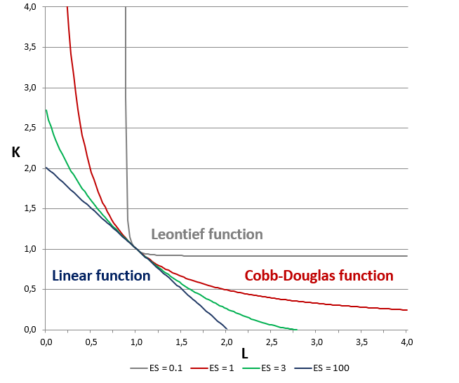
Depending on the assumed degree of substitution between inputs, special cases of the CES production function are:
- The linear production function where inputs are perfect substitutes. The elasticity of substitution between input tend to infinity. Capital (\(K\)) can be substituted for labor (\(L\)) perfectly. Isoquants that represent all the combination of capital and labor required to produce a given quantity of output (\(Q\)) are straight lines.
- The Cobb-Douglas function where the elasticity of substitution between inputs is equal to one. The isoquants are curved with a slope changing along them, indicating that labor and capital are not perfect substitutes.
- The Leontief production function where inputs are perfect complements. The elasticity of substitution between inputs is zero. In this case, the isoquants are right angles (L shaped). Inputs cannot be substituted from one to another. Capital and labor can only be used in fixed proportions.
graphique 2 represents graphically different CES production functions for various elasticities of substitution.
Assuming a CES production function, the constrained cost minimization program is :
\[ min_{x_i} \sum_{i=1}^{n} p_i.x_i \]
\[ \ s.t \ Q= Q(x_i)= \sum_{i=1}^{n} (\Phi_i.x_i^{\frac{\rho-1}{\rho}})^{\frac{\rho}{\rho-1}}\]
where \(\rho\) is the elasticity of substitution between inputs and \(x_i\) the efficient input \(i\) (including technical progress)
The resolution of this program allows for deriving the demand for production factors expressed as follows (see Proof at the end of this section):
\[ x_i= Q.(\Phi_i)^{\rho}.(\frac{p_i}{p})^{-\rho} \]
\[ P= (\sum_{i=1}^{n} (\Phi_i)^{\rho}.(p_i)^{1-\rho})^{\frac{1}{1-\rho}} \]
Where \(P\) is the Dixit et Stiglitz (1977) input price index.
In the case of two inputs (labor and capital) and taking input account technical progress, the demand for labor (L) and for capital (K\(^{CES}\)) that will be used later in our CGE model (Equation équation 4 and équation 5) are defined as follows:
\[L = \left( \frac{Y}{PROG^{L}} \right) . \left( \left( \varphi^{L} \right) ^ {\rho} \right) . \left( \frac{w}{\left( p . PROG^{L} \right)} \right) ^ {\left( -\rho \right)}\]
\[K^{CES} = \left( \frac{Y}{PROG^{K}} \right) . \left( \left( \varphi^{K} \right) ^ {\rho} \right) . \left( \frac{\left( \delta + r \right)}{PROG^{K}} \right) ^ {\left( -\rho \right)}\]
Proof. Solution based on the Lagrangian multipliers
\[ \mathcal{L} = min_{x_i} \sum_{i=1}^{n} p_i.x_i - \lambda.[Q-Q(x_i)] \\ \dfrac{\partial \mathcal{L}}{\partial x_i} = 0 \Longleftrightarrow p_i + \lambda \dfrac{\partial {Q}}{\partial Q(x_i)} = 0\\ \Longleftrightarrow \lambda = \frac{-p_i}{Q'(x_i)} \\\]
At the optimum, the ratio between the marginal productivity of two inputs is equal to their relative price:
\[\frac{Q'(x_i)}{Q'(x_j)} = \frac{p_i}{p_j} \\ \dfrac{\partial \mathcal{L}}{\partial \lambda} = 0 \Longleftrightarrow Q = Q(x_i) \\ Q'(x_i) = \Phi_i. (\frac{x_i}{Q})^{\frac{-1}{\rho}} \\ \frac{Q'(x_i)}{Q'(x_j)} = \frac{\Phi_i}{\Phi_j}. (\frac{x_i}{x_j})^{\frac{-1}{\rho}} =\frac{p_i}{p_j}\\ \Phi_i.(x_i)^{\frac{-1}{\rho}} = \frac{p_i}{p_j}. Q_j. x_j^{\frac{-1}{\rho}} \\ \Phi_i.(x_i)^{1-\frac{1}{\rho}} = \frac{p_i.x_i}{p_j.x_j}.\Phi_j.x_j^{1-\frac{1}{\rho}}\\ Q^{\frac{\rho-1}{\rho}}= \Phi_j.x_j^{1-\frac{1}{\rho}}[\frac{\sum_{i=1}^{n} p_i.x_i}{p_j.x_j}]\\ \ Assume \ P.Q = \sum_{i=1}^{n} p_i.x_i \\ Q^{1-\frac{1}{\rho}}= \Phi_j.x_j^{1-\frac{1}{\rho}}.[\frac{P.Q}{p_j.x_j}]\\ x_j= Q.\Phi_j^{n}.(\frac{p_j}{P})^{-\rho} \\ P=\sum_{i=1}^{n} p_i.\frac{x_i}{Q} = \sum_{i}^{n} p_i.\Phi_i^{\rho}.(\frac{p_i}{P})^{-\rho} \\ P= [\sum_{i=1}^{n} \Phi_i^{\rho}.p_i^{1-\rho}]^{\frac{1}{1-\rho}}\]
2.1.3 Households’ consumption
We shall start with a simple model to describe the consumption behaviour. We consider that households supply labor and capital, for which they get their income (\(w.L + p.r.k\)) . We assume that households wish to use a fixed share of their total income for consumption:
\[CH = \left( 1 - \sigma \right) . \frac{\left( w . L + p . r . K \right)}{p}\]
The above consumption equation can derived from various microeconomic optimizing behaviour. We propose a simple one below. Let us assume that the consumer maximize its utility by allocating the income of a given periods over several periods. The optimizing program is:
\[ max_{c_i} U(c_1, c_2, ... c_n)=\sum_{i=1}^{n} (\phi_i.c_i^{\frac{\rho-1}{\rho}})^{\frac{\rho}{\rho-1}} \]
\[ \ s.t \ \sum_{i=1}^{n} p_i.c_i = R \]
where \(\rho\) is the elasticity of substitution, \(c_i\) the consumption of good \(i\) and \(R\) total income.
The resolution of this program gives the relationship between households consumption and total income (see Proof below):
\[ p_i.c_i= (\Phi_i)^{\rho}.(\frac{p_i}{P})^{1-\rho}.R \]
with \((\Phi_i)^{\rho}.(\frac{p_i}{P})^{1-\rho}\) the consumption share.
\[P= (\sum_{j=1}^{n} (\Phi_j)^{\rho}.(P_j)^{1-\rho})^{\frac{1}{1-\rho}}\]
Proof. Solution based on the Lagrangian multipliers
\[ \mathcal{L} = \sum_{i=1}^{n} (\phi_i.c_i^{\frac{\rho-1}{\rho}})^{\frac{\rho}{\rho-1}} - \lambda.[\sum_{i=1}^{n} p_i.c_i - R] \\ \dfrac{\partial \mathcal{L}}{\partial c_i} = 0 \Longleftrightarrow \dfrac{\partial {U}}{\partial U(c_i)} - \lambda.p_i\\ \Longleftrightarrow \lambda = \frac{U'(c_i)}{p_i} \\\]
At the optimum, the ratio between the marginal productivity of two inputs is equal to their relative price:
\[ \frac{U'(c_i)}{U'(c_j)} = \frac{p_i}{p_j} \\ \dfrac{\partial \mathcal{L}}{\partial \lambda} = 0 \Longleftrightarrow \sum_{i=1}^{n} p_i.c_i = R \\ U'(c_i) = \Phi_i. (\frac{c_i}{U})^{\frac{-1}{\rho}} \\ \frac{c_i}{c_j} = (\frac{\Phi_i}{\Phi_j}) ^ {\rho}. (\frac{p_i}{p_j})^{-\rho} \\ \frac{p_i.c_i}{p_j.c_j} = (\frac{\phi_i}{\phi_j})^{\rho}. (\frac{p_i}{p_j})^{1-\rho} \\ p_j.c_j = (\frac{\phi_j}{\phi_i})^{\rho}.(\frac{p_j}{p_i})^{1-\rho}.p_i.c_i\\ (\frac{\phi_1}{\phi_i})^{\rho}.(\frac{p_1}{p_i})^{1-\rho}.p_i.c_i + (\frac{\phi_2}{\phi_i})^{\rho}.(\frac{p_2}{p_i})^{1-\rho}.p_i.c_i+ ...+ (\frac{\phi_j}{\phi_i})^{\rho}.(\frac{p_j}{p_i})^{1-\rho}.p_i.c_i +... = R\\ p_i.c_i.(\frac{1}{(\phi_i)^{\rho}.(p_i)^{1-\rho}}).\sum_{j=1}^{n} (\phi_j)^{\rho}.(p_j)^{1-\rho} = R\\ \ Assume \ P.C = \sum_{j=1}^{n} p_j.c_j \\ P^{1-\rho}=\sum_{j=1}^{n} (\phi_j)^{\rho}.(p_j)^{1-\rho} \Longrightarrow P= (\sum_{j=1}^{n} (\phi_j)^{\rho}.(p_j)^{1-\rho})^{\frac{1}{1-\rho}}\\ p_i.c_i = (\phi_i)^{\rho}.(\frac{p_i}{P})^{1-\rho}.R \]
This general result is based on the assumption that the consumer maximizes its utility by allocating its income over several periods. If we consider a simplified case with only two periods: \(i=1\) (present) and \(i=2\) (future):
\[ p_1.c_1 = (\phi_1)^{\rho}.(\frac{p_1}{P})^{1-\rho}.R \]
Assuming a CES function with \(\rho=1\), we find that consumption is a constant share of income :
\[ p_1.c_1 = \phi_1.R \]
with \(\phi_1\) = (1-\(\sigma\)) and \(\sigma\) the propensity to save.
3 Identities and definitions
3.1 Production: Supply-Demand Equilibrium
This equation is the market equilibrium condition between supply and demand. The equation of production is an accounting one and does not require derivation. It states that everything that is being produced (total supply) is “consumed”, either by household’s consumption, investment or government spending (total demand):
\[Y = CH + I + G\]
3.2 Capital accumulation
Given an initial capital stock (at \(t-1\)), the change in capital stock defines the capital stock in \(t\):
\[\varDelta \left(K\right) = I_{t-1} - \delta . K_{t-1}\]
By definition, the change in capital stock depends on two items:
- It increases with the investment made in the previous period (\(I_t-1\))
- It decreases with the depreciation of the capital stock (\(\delta.K_t-1\))
3.3 Cost of capital
We assume that the cost of capital is defined according to the standard specification of the user cost of capital (or real rental price of capital services or the costs of holding capital) proposed in the literature (see e.g. Chap.9 Jorgenson (1963), Romer (2016)):
\[ c^{K} = p(\delta + r) \]
where \(\delta\) is the depreciation rate of capital, \(r\) the interest rate and \(p\) the price of the investment.
The above equation may have several interpretations. A first one is that it reflects the opportunity cost of holding capital, that is the cost of not been able to invest an existing financial wealth into another asset. A second one is to assume that capital is financed through bank credit and that the reimbursement of the debt corresponds to the depreciation of capital. The underlying idea is that the loan cannot exceed the duration of the equipment. In this case the cost of capital corresponds to the annuities paid by the firm (reimbursement of the debt plus interests paid).
4 Annexes
4.1 Endogenous variables’ equations
Production (GDP) \[Y = CH + I + G \tag{1}\]
This equation is an identity or accountancy relation. \
Price \[p . Y = w . L + p . \left( \delta + r \right) . K \tag{2}\]
Households consumption \[CH = \left( 1 - \sigma \right) . \frac{\left( w . L + p . r . K \right)}{p} \tag{3}\]
Labor demand \[L = \left( \frac{Y}{PROG^{L}} \right) . \left( \left( \varphi^{L} \right) ^ {\rho} \right) . \left( \frac{w}{\left( p . PROG^{L} \right)} \right) ^ {\left( -\rho \right)} \tag{4}\]
This equation is derived from a cost minimization assuming a CES production function technology. \
Capital demand (from CES function) \[K^{CES} = \left( \frac{Y}{PROG^{K}} \right) . \left( \left( \varphi^{K} \right) ^ {\rho} \right) . \left( \frac{\left( \delta + r \right)}{PROG^{K}} \right) ^ {\left( -\rho \right)} \tag{5}\]
Capital (from accumulation equation) \[\varDelta \left(K\right) = I_{t-1} - \delta . K_{t-1} \tag{6}\]
4.2 Glossary of variables
| \(CH\) | Households consumption | 3 |
| \(K\) | Capital (from accumulation equation) | 6 |
| \(K^{CES}\) | Capital demand (from CES function) | 5 |
| \(L\) | Labor demand | 4 |
| \(p\) | Price | 2 |
| \(Y\) | Production (GDP) | 1 |
Bibliograhie
Réutilisation
Citation
@article{untitled,
  author = {},
  title = {Chapter 1: Introduction to CGE model},
  url = {https://www.ofce.fr/qmd_cge_theory/Manual/Ch01.html},
  langid = {fr}
}