Micro-economic foundations
Micro-economic foundations
PLots Walrasian closure (overleaf)
Behavior equations versus identities
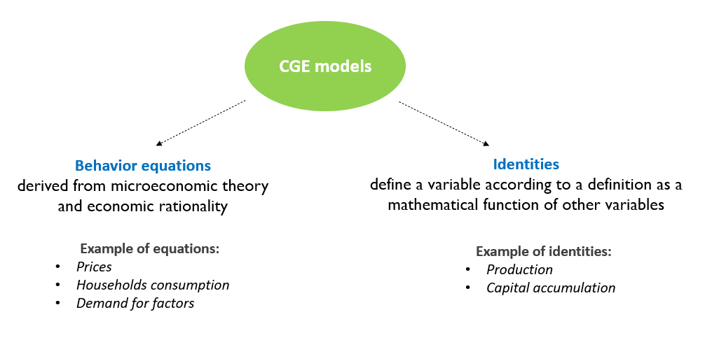
- CGE models have behavioral and identity equations
- Behavioral equations derive from microeconomic theory and economic rationality
- Economic behavior of producers, consumers, and other agents in the model
- Identity equations define a variable according to a definition as a mathematical function (sum, product, etc.) of other variables
- Accountancy variables (e.g. GDP, price index), unemployment rate, etc.
![]()
Behavior equations
Prices
We assume oligopolistic competition à la Cournot where each producer defines its price in order to maximize its profit considering the price of the other producers as given:
The maximisation program is:
\[\begin{equation}
max_y Π(y) = p(y).y - c(y)
\end{equation}\]
where \(y\) is the production or demand adressed to the compagny, \(\pi(y)\) is the profit of the compagny, \(p(y)\) its price and \(c(y)\) the production cost. We assume \(p′(y)\) < 0, \(c′(y)\) > 0 and \(c′′(y)\) > 0
- The result of the program maximization defines the optimum price that is equal to a markup over the production costs:
\[\begin{equation}
p(y)= [1+ m^{up}].c'(y)
\end{equation}\]
where the markup is: \[\begin{equation} m^{up}= 1/(\epsilon -1) \end{equation}\] and \(\epsilon\) the (absolute) price elasticity of demand
In perfect competition, markup is zero: \[\begin{equation} m^{up} = 0 \end{equation}\] so that the optimal price is equal to the marginal cost of production: \[\begin{equation} p(y)= c'(y) \end{equation}\]
Given that production costs equal total factor payments, the optimal price is therefore equal to the cost of capital and labor:
\[\begin{equation}
p(y).y= w.L+ p(\delta+r).K
\end{equation}\]
Households consumption
We assume that households supply labor and own the capital, for which they get their income (\(w.L + p.r.K\)) .
We assume that households wish to use a fixed share of their total income for consumption
\[\begin{equation}
CH = \left( 1 - \sigma \right) . \frac{\left( w . L + p . r . K \right)}{p}
\end{equation}\]
The consumer maximize its utility by allocating the income of a given period over several periods.
The maximization program is:
\[\begin{equation}
max_{c_i} U(c_1, c_2, ... c_n)=\sum_{i=1}^{n} (\phi_i.c_i^{\frac{\rho-1}{\rho}})^{\frac{\rho}{\rho-1}}
\end{equation}\]
\[\begin{equation}
\ s.t \ \sum_{i=1}^{n} p_i.c_i = R
\end{equation}\] where \(\rho\) is the elasticity of substitution, \(c_i\) the consumption of good \(i\) and \(R\) total income.
The resolution of this program gives the relationship between households consumption and total income :
\[\begin{equation}
p_i.c_i= (\Phi_i)^{\rho}.(\frac{p_i}{P})^{1-\rho}.R
\end{equation}\] where \((\Phi_i)^{\rho}.(\frac{p_i}{P})^{1-\rho}\) is the consumption share.
Considering only two periods: \(i=1\) (present) and \(i=2\) (future) and assuming a CES function with \(\rho=1\), we find that consumption is a constant share of income:
\[\begin{equation*}
p_1.c_1 = \phi_1.R
\end{equation*}\] with \(\phi_1\) = (1-\(\sigma\)) and \(\sigma\) the propensity to save.
Demand for production factors
The firm determines its demand for labor and capital by maximizing its profit, which is equivalent to minimizing its production cost taking into account the production function.
Assuming a CES production function, the constrained cost minimization program is:
\[\begin{equation}
min_{x_i} (\sum_{i=1}^{n} p_i.x_i) \\
s.t \\ Q= Q(x_i) = (\sum_{i=1}^{n} \Phi_i.x_i^{(\frac{\rho-1}{\rho})})^{(\frac{\rho}{\rho-1})}
\end{equation}\]
where \(\rho\) is the elasticity of substitution between inputs.
- The resolution of the program derives demand for factors expressed as follows:
Labor demand:
\[\begin{equation}
L = \left( \frac{Y}{PROG^{L}} \right) . \left( \left( \varphi^{L} \right) ^ {\rho} \right) . \left( \frac{w}{\left( p . PROG^{L} \right)} \right) ^ {\left( -\rho \right)}
\end{equation}\]
Capital demand:
\[\begin{equation}
K = \left( \frac{Y}{PROG^{K}} \right) . \left( \left( \varphi^{K} \right) ^ {\rho} \right) . \left( \frac{\left( \delta + r \right)}{PROG^{K}} \right) ^ {\left( -\rho \right)}
\end{equation}\]
Identities and defnitions
Production
\[\begin{equation}
Y = CH + I + G
\end{equation}\]
- Market equilibrium condition between supply and demand
- Accountancy equation that states that everything that is being produced (total supply) is “consumed”, either as household’s consumption, investment or government spending (total demand)
Capital accumulation
- Given an initial capital stock (at \(t-1\)), the change in capital stock defines the capital stock in \(t\):
\[\begin{equation}
\varDelta \left(K\right) = I_{t-1} - \delta . K_{t-1}
\end{equation}\]
- The change in capital stock :
- Increases with the investment made in the previous period (\(I_{t-1}\))
- Decreases with the depreciation of the capital stock (\(\delta.K_{t-1}\))
Cost of capital
We assume that the cost of capital is defined as the user cost of capital (or real rental price of capital services or the costs of holding capital) :
\[\begin{equation}
c^{K} = p(\delta + r) \\
\end{equation}\]
where \(\delta\) is the depreciation rate of capital, \(r\) the interest rate and \(p\) the price of the investment.
- This equation may have several interpretations:
- It reflects the opportunity cost of holding capital, that is the cost of not been able to invest an existing financial wealth into another asset
- It assumes that capital is financed through bank credit and that the reimbursement of the debt corresponds to the depreciation of capital
Some definitions
- Endogenous variable: defined inside the model, as a result of the model simulation
- One equation for each endogenous variable
- Eg. production, consumption, prices, wages, etc.
- Exogenous variable: defined outside the model
- No equation in the model defining this variable: hypothesis of the model
- Eg. population, price of imports (for a one country model)
- Parameter: from a mathematical point of view, an exogenous variable that is generally constant
- Eg. elasticities (substitution, indexation, etc.), depreciation rate, tax rate, etc.
- Representative agent: an average relevant economic agent that follows an optimizing/rational economic behaviour
- Households, producers, government
- Optimize an objective: e.g. maximization of profit/utility/social welfare, minimization of cost
Macroeconomic closure
- A model is a way of explaining endogenous variables as function of exogenous variables.
- Making a choice of what is to be determined within the model (endogenous variables) and what is to be considered external to the model (exogenous variables) is called the model closure . Why does the choice of the model closure matter?
- It may define the direction of causality (which variables determine the others)
- It may have important implications on the properties and results of the model
What is the impact of an increase in public spending (multiplier of public expenditures) on the endogenous variables of the model depending on the choice of the closure ?
We compare the results for two contrasting model closures:
- The Walrasian model . The model is found in ThreeME-R-training/src/model/training/02.1-eq.mdl . It is called in the « config_training.R » file in the section « Model files ».
- The Keynesian model . The model is found in ThreeME-R-training/src/model/training/02.2-eq.mdl . It is called in the « config_training.R » file in the section « Model files ».
Walrasian versus Keynesian models
Common features for both models :
- General equilibrium : which means that supply equals demand in all markets.
- In both frameworks, the models consist of equations that solve for the endogenous variables, given the exogenous variables and parameters. A change in one or more exogenous variable or parameter will lead to adjustments in the endogenous variables so to solve the system of equations again. These solved values of all endogenous variables, constitute the outcome of the model .
Main difference between both models:
- The choice of endogenous variables . In the Walrasian framework some variables adjust while there are considered fixed in the Keynesian framework and vice-versa.
Note: Our definitions of the Walrasian and Keynesian closures may differ from those found in the literature inspired by the seminal work of Sen (1963). Contrary to this literature that consider a static case, we propose simulations based on a dynamic model including an equation for capital accumulation and where investment is endogenous in both the Walrasian and the Keynesian closure.
The Walrasian model
The model is based on a set of 7 equations with 7 endogenous variables:
Investment
\[\begin{equation}
I = Y - CH - G
\end{equation}\]
Production
\[\begin{equation}
Y . p = w . L + p . \left( \delta + r \right) . K
\end{equation}\]
Households’consumption
\[\begin{equation}
CH = \left( 1 - \sigma \right) . \frac{\left( w . L + p . r . K \right)}{p}
\end{equation}\]
Wage
\[\begin{equation}
w + L = \left( \frac{Y}{PROG^{L}} \right) . \left( \left( \varphi^{L} \right) ^ {\rho} \right) . \left( \frac{w}{\left( p . PROG^{L} \right)} \right) ^ {\left( -\rho \right)} + w
\end{equation}\]
Interest rate
\[\begin{equation}
r + K = \left( \frac{Y}{PROG^{K}} \right) . \left( \left( \varphi^{K} \right) ^ {\rho} \right) . \left( \frac{\left( \delta + r \right)}{PROG^{K}} \right) ^ {\left( -\rho \right)} + r
\end{equation}\]
Capital (from accumulation equation)
\[\begin{equation}
\varDelta \left(K\right) = I_{t-1} - \delta . K_{t-1}
\end{equation}\]
Price
\[\begin{equation}
p=1
\end{equation}\]
The price equation defines the price as numéraire (equal to 1). The price can therefore be seen as an exogenous variable. The model could be written as a set of 6 equations with 6 endogenous variables.
The Keynesian model
The model is based on a set of 6 equations with 6 endogenous variables:
\[\begin{equation}
Y = CH + I + G
\end{equation}\]
\[\begin{equation}
p . Y = w . L + p . \left( \delta + r \right) . K^{n}
\end{equation}\]
\[\begin{equation}
CH = \left( 1 - \sigma \right) . \frac{\left( w . L + p . r . K \right)}{p}
\end{equation}\]
\[\begin{equation}
L = \left( \frac{Y}{PROG^{L}} \right) . \left( \left( \varphi^{L} \right) ^ {\rho} \right) . \left( \frac{w}{\left( p . PROG^{L} \right)} \right) ^ {\left( -\rho \right)}
\end{equation}\]
- Capital (notional level from cost minimization of a CES function )
\[\begin{equation}
K^{n} = \left( \frac{Y}{PROG^{K}} \right) . \left( \left( \varphi^{K} \right) ^ {\rho} \right) . \left( \frac{\left( \delta + r \right)}{PROG^{K}} \right) ^ {\left( -\rho \right)}
\end{equation}\]
- Capital (effective level from capital accumulation)
\[\begin{equation}
\varDelta \left(K\right) = I_{t-1} - \delta . K_{t-1}
\end{equation}\]
\[\begin{equation}
\varDelta \left(\operatorname{log} I\right) = \varDelta \left(\operatorname{log} K^{n}_{t-1}\right) + \alpha^{I,Kn} . \operatorname{log} \frac{K^{n}_{t-1}}{K_{t-1}}
\end{equation}\]
To go further
Micro-economic foundations
PLots Walrasian closure (overleaf)
Practice: Equivalence of results with alternative specifications (Walrasian case)
Let’s replace the initial specification of of some functions in the equation file 02.1-eq.mdl file by alternative specifications and see how the results change.
You can change the specification of the model by activating or deactivating certain equations
- The # symbol is used to comment a line
- Omit the # symbol in front of the wanted equation and add the # symbol in from of the to the one you don’t want to read
Run the model using the following alternative specifications:
Production
\[\begin{equation}
Y = \left( \left( \varphi^{L} . L ^ {\left( \frac{\left( \rho - 1 \right)}{\rho} \right)} \right) + \left( \varphi^{K} . K ^ {\left( \frac{\left( \rho - 1 \right)}{\rho} \right)} \right) \right) ^ {\left( \frac{\rho}{\left( \rho - 1 \right)} \right)}
\end{equation}\]
- This is the CES production function. Can be obtained by inserting the inverse demand function into the production equation (Walras model)
Household’s consumption \[\begin{equation}
\varDelta \left(\operatorname{log} CH\right) = \varDelta \left(\operatorname{log} Y_{t-1}\right)
\end{equation}\]
Inverse factor demand functions
\[\begin{equation}
\frac{w}{\left( p . PROG^{L} \right)} = \varphi^{L} . \left( \frac{Y}{\left( L . PROG^{L} \right)} \right) ^ {\left( \frac{1}{\rho} \right)}
\end{equation}\]
\[\begin{equation}
\frac{\left( r + \delta \right)}{PROG^{K}} = \varphi^{K} . \left( \frac{Y}{\left( K . PROG^{K} \right)} \right) ^ {\left( \frac{1}{\rho} \right)}
\end{equation}\]
- Check that the results are equivalent to the previous specifications.
Practice: Explosive dynamics with the Keynesian model
Change in the 02.1-calib.mdl file the value of the adjustment parameter of investment to notional capital from \(\alpha_{I}^{Kn}\) = 0.1 to \(\alpha_{I}^{Kn}\) = 0.6
Accounting for economic growth
Previously we make the assumption of a steady state economy where the growth rate of volume and price variables are zero. This requires the assumptions that in the long term the growth rate of technical progress and of the population is zero.
Now let’s assume a growing economy.

1.8 Comments on the Walrasian model closure
Note: we consider a steady state economy (with growth rate = 0%)